
시계열 분석 part1 - Auto-Regressive, Moving-Average
시계열 데이터는 일정 시간동안 수집된 일련의 데이터로, 시간에 따라서 샘플링되었기 때문에 인접한 시간에 수집된 데이터는 서로 상관관계가 존재하게 됩니다. 따라서 시계열 데이터를 추론하는데, 전통적인 통계적 추론이 적합하지 않을수 있습니다. 현실 세계에서는 날씨, 주가, 마케팅 데이터 등등 다양한 시계열 데이터가 존재하고, 시계열 분석을 통해 이러한 데이터가 생성되는 메카니즘을 이해하여 설명가능한 모델로서 데이터를 표현하거나, 미래 값을 예측하는 것, 의미있는 신호값만만 분리하는 일에 활용할 수 있습니다.
일반적인 시계열분석의 과정은 아래와 같습니다.
- Plot the series and examine the main features of the graph, checking in particular whether there is
- A trend
- A seasonal component
- Any apparent sharp changes in behavior
- Any outlying observations
- Remove the trend and seasonal components to get stationary residuals
- To achieve goal, you may need to apply a preliminary transformation like taking logarithms
- Estimate the trend and seasonal components using classical decomposition model
- Or Eliminate the trend and seasonal components using differencing
- Anyway, the goal is to get stationary residuals
- Choose a model to fit the residuals
- Forecasting the residuals and then inverting the transformations for original series
- Alternative approach is to express the series in terms of its Fourier components. But it will not be discussed in here.
시계열 분석은 시간의 경과에 따라 변하지 않는 어떤 특성을 가진 프로세스를 분석하는 것입니다. 만약 시계열 데이터를 예측하고자 한다면, 우리는 시간에 따라 변하지 않는 무언가가 있다는 것을 반드시 가정해야합니다. 예를 들면 평균이 변하지 않는것(no trend), 분산이 변하지 않고, 주기적인 패턴이 없는 데이터를 가정합니다. 이러한 속성을 “stationary”하다고 합니다. 어떤 시계열 데이터가 stationary하다는 가정을 하면, 우리는 다양한 기법들을 활용할수 있습니다. 앞으로의 포스팅에서는 이러한 기법들이 무엇인지 소개하려고 합니다.
Stationary, Auto-Covariance Function and Auto-Correlation Function
시계열 \(\{X_t, t=0, \pm 1, ...\}\) 가 stationary하다는 것은 h lag만큼 time-shifted 된 시계열 \(\{X_{t+h}, t=0, \pm 1, ...\}\)와 통계적인 속성이 유사하다는 것을 의미합니다. 이 때 통계적인 속성을 first and second order moments(mean and covariance)로만 제한하면, 아래와 같이 수식적 정의를 할 수 있습니다.
Definition
Let \({X_t}\) be a time series with \(E(X_t^2) < \infty\).
The mean function of \({X_t}\) is \(\mu_X(t) = E(X_t)\).
The covariance function of \({X_t}\) is \(\rho_X(r, s) = Cov(X_r, X_s) = E[(X_r - \mu_X(r))(X_s - \mu_X(s))]\) for all integers r and s.
Definition
\({X_t}\) is (weakly) stationary if
1) \(\mu_X(t)\) is independent of t.
2) \(\gamma_X(t+h, t)\) is independent of t for each h.
Strictly stationary is also
3) \((X_1, ..., Xn)\) and \((X_{1+h}, ..., X_{n+h})\) have the same joint distributions for all h and n >0
2)에서의 정의를 이용해 stationary한 타임시리즈의 \(\gamma_X(t+h, t)\)는 t에 대해서 무관하기 때문에 \(\gamma(\cdot)\)는 “autocovariance function”으로 부르며, \(\gamma_X(h)\)는 h lag에서의 값을 지칭하는 것으로 하겠습니다. 또한 covariance를 normalization하여 correlation을 함께 정의할수 있습니다.
Definition
Let \({X_t}\) be a stationary time series.
The autocovariance function (ACVF) of \({X_t}\) at lag h is \(\gamma_X(h) = Cov(X_{t+h}, X_t)\).
The autocorrelation function (ACF) of \({X_t}\) at lag h is \(\rho_X(h) \equiv \frac{\gamma_X(h)}{\gamma_X(0)} = Cor(X_{t+h}, X_t)\)
stationary time series의 대표적인 예는 iid noise와 white noise가 있습니다. iid noise는 \(\{X_t\}\)가 동일하고(identically) 서로 독립적인(independent) 분포를 따르며, 평균이 0인 확률변수로 정의됩니다. t에 상관없이 평균이 0이고, \(\gamma_X(\cdot)\)도 0이기때문에 stationary 조건을 만족합니다.
\[\begin{align} \gamma_X(t+h, t) & = \sigma^2, \ & if \ h=0 \\ & = 0, \ & if \ h \ne 0 \end{align}\]마찬가지로 white noise with zero mean and variance \(\sigma^2\)도 (weak) staionary 조건을 만족합니다. 참고로 iid noise와 white noise는 다릅니다. 모든 iid noise는 white noise이지만, 그 역은 성립하지 않습니다. 참고
시계열 데이터(realization)가 주어졌을때, 이 프로세스의 mean과 covariance를 추정하기 위해 sample mean과 sample covariance function, sample autocorrelation function를 사용합니다.
Definition
Let \(x_1, ..., x_n\) be observations of a time series.
The sample mean of \(x_1, ..., x_n\) is \(\bar{x} = \frac{1}{n} \sum_{t=1}^n x_t\)
The sample autocovariance function is \(\hat{\gamma} := n^{-1} \sum_{t=1}^{n-|h|}(x_{t+|h|} - \bar{x})(x_{t} - \bar{x}), -n < h < n\)
The sample autocorrelation function is \(\hat{\rho} := \frac{\hat{\gamma}(h)}{\hat{\gamma}(0)}, -n < h < n\)
Moving Average and Auto Regressive process
시계열 분석의 문제는 stocastic process의 realization인 시계열 데이터 \(\{X_t\}\)가 주어졌을때(그리고 \(\{X_t\}\)가 stationary할때), 우리는 이 데이터가 생성된 본래의 stocastic process를 모델링하고 싶다는 겁니다. 데이터가 주어져있기때문에 우리는 (sample) mean과 lag에 따른 covariance과 correlation은 쉽게 구할수 있는 상황입니다.(auto covariance function과 auto correlation function)
만약 ACF가 주어졌을때 이에 대응되는 stationary stochatic process가 unique하게 결정된다면 아주 쉬운 문제가 됩니다. analytic한 솔루션이 1개 존재하는 것이고, 그건 공식에 맞춰 계산하면 되는 문제가 되니까요. 그러한 특징과 관련된 2가지 모델을 살펴보도록 하겠습니다.
The MA(q) process:
\(\{X_t\}\) is a moving-average process of order q if
\(X_t = Z_t + \theta_1 Z_{t-1} + ... + \theta_q Z_{t-q}\)
where \(\{Z_t\} \sim WN(0, \sigma^2)\) and \(\theta_1, ..., \theta_q\) are constants.
\(\{X_t\}\)가 t 이전 시점의 white noise \(\{Z_x\}\)(s \(\le\) t)로 표현되는 프로세스를 Moving Average process라고 합니다. 앞서 본 “stationary” 정의에 따라, MA(q) process는 항상 (weakly) stationary합니다.
invertibility :
흥미롭게도 MA(1)은 AR(\(\infty\))로 변환될수 있습니다. 아래 수식에서 볼수 있듯이 \(Z_t\)는 \(X_t\)의 과거값들의 linear combination로 표현될수 있습니다.
\[\begin{align} X_t & = Z_t + \theta Z_{t-1} \\ Z_t & = X_t - \theta Z_{t-1} \\ & = X_t - \theta(X_{t-1} - \theta Z_{t-2}) \\ & = X_t - \theta X_{t-1} + \theta^2 (X_{t-2} - \theta Z_{t-3}) \\ & = X_t - \theta X_{t-1} + \theta^2 X_{t-2} - \theta^3 X_{t-3} + ... + (-\theta)^n Z_{t-n}, & when \left\vert \theta \right\vert \lt 1, (-\theta)^n Z_{t-n} \approx 0 \\ & = \sum_{n=0}^{\infty} (-\theta)^nX_{t-n} \\ \end{align}\]이러한 성질을 일반화하여 MA(q)에 대해 이야기할 수 있습니다. white noise인 \(Z_t\)를 \(X_t\)의 무한등비급수의 형태로 표현할수 있다면, 주어진 \(\{X_t\}\)는 invertible하다고 정의합니다. 이 때 수렴 조건(MA(1)에서의 \(\left\vert \theta \right\vert \lt 1\))을 invertibility condition이라고 하고 합니다.
\[\begin{align} Z_t & = \theta(B)X_t, \ & where \ \theta(\cdot) \ are \ the \ q-th \ degree \ polynomials \\ \theta(z) & = 1 + \theta z + ... + \theta_q z^q \end{align}\]자세한 증명은 여기서 다루지 않지만, 결론적으로는 \(\theta(z)\)의 해가 unit circle 밖에 있는 경우 invertible 조건을 만족하게 됩니다.
Invertibility is equivalent to the condition
\[\theta(z) = 1+ \theta_1 z + ... + \theta_q z^q \ne 0 \ for \ all \left\vert z \right\vert \le 1\]invertible이 중요한 이유는 ACF가 주어질 때, 이 ACF를 만족하는 MA process가 unique하게 결정되기 때문입니다.
두번재 모델은 Auto-Regressive Process입니다. \(\{X_t\}\)가 이전 시점의 자기 자신 값 \(\{X_s\}\)(s \(\le\) t)와 t 시점의 white noise \(\{Z_x\}\)로 표현되는 프로세스를 Auto-Regress process라고 합니다. 기억해야할 점은 MA process와 달리 AR process는 항상 stationary한 것은 아니라는 점입니다.
The AR(q) process:
\(\{X_t\}\) is a auto-regressive process of order q if
\(X_t = Z_t + \phi_1 X_{t-1} + ... + \phi_q X_{t-q}\)
where \(\{Z_t\} \sim WN(0, \sigma^2)\) and \(\phi_1, ..., \phi_q\) are constants
MA process의 invertibility 와 유사한 개념으로 AR process에 casuality 개념을 도입할수 있습니다. 아래는 AR(1) process를 MA(\(\infty\))로 변환하는 예시입니다.
\[\begin{align} X_t & = \phi X_{t-1} + Z_t \\ & = \phi (\phi X_{t-2} + Z_{t-1}) + Z_t \\ & = \phi^2 X_{t-2} + \phi Z_{t-1} + Z_t \\ & = \phi^2 (\phi X_{t-3} + Z_{t-2}) + \phi Z_{t-1} + Z_t \\ & = Z_t + \phi Z_{t-1} + \phi^2 Z_{t-3} + ... + \phi^n X_{t-n}, & when \left\vert \phi \right\vert \lt 1, \phi^n X_{t-n} \approx 0 \\ & = \sum_{n=0}^{\infty} (\phi)^n Z_{t-n} \\ \end{align}\]\(X_t\)를 white noise인 \(Z_x\)(단, s \(\le\) t)의 linear combination 형태로 표현된다면, 주어진 \(\{X_t\}\)는 causal하다고 정의합니다. 위의 예시인 AR(1) process \(\{X_t\}\)가 causal하기 위해서는 \(\left\vert \phi \right\vert \lt 1\) 입니다.
이러한 성질을 일반적인 AR(p) process에 대해서도 이야기할수 있습니다.
\[\begin{align} X_t & = \phi(B)X_t, \ & where \ \phi(\cdot) \ are \ the \ p-th \ degree \ polynomials \\ \phi(z) & = 1+ \phi z + ... + \phi_p z^p \end{align}\]자세한 증명은 여기서 다루지 않지만, 결론적으로는 \(\phi(z)\)의 해가 unit circle 밖에 있는 경우 causality 조건을 만족하게 됩니다.
Causality is equivalent to the condition
\[\phi(z) = 1 + \phi_1 z + ... + \phi_p z^p \ne 0 \ for \ all \left\vert z \right\vert \le 1\]중요한 것은 causality를 만족하는 AR(p) process는 항상 stationary하고, stationary AR(p) process는 항상 causality를 만족합니다.
ARMA(p, q)
AR(p)와 MA(q)가 합쳐진 process를 ARMA(p, q)로 표기하고 ARMA(p,q) process가 유일한 stationary solution \(\{X_t\}\)를 갖는 조건은 causality condition을 만족할 때이며, 그 역도 성립합니다.
Definition
\(\{X_t\}\) is an ARMA(p, q) process if \(\{X_t\}\) is stationary and if for every t,
\[X_t - \phi_1 X_{t-1} - ... - \phi_p X_{t-p} = Z_t + \theta_1 Z_{t-1} + ... + \theta_q Z_{t-q}\]where \(\{Z_t\} \sim WN(0, \sigma^2)\) and the polynomials \(( 1 - \phi z - ... - \phi_p z^p)\) and \((1+\theta_1 z + ... + \theta_q z^q )\) have no common factors.
Existence and Uniqueness :
A stationary solution \(\{X_t\}\) of equation ARMA(p, q) exists (and is also the unique stationary solution) if and only if
\[\phi(z) = 1 + \phi_1 z + ... + \phi_p z^p \ne 0 \ for \ all \left\vert z \right\vert \le 1\]Example
아래와 같은 조건을 만족하는 ARMA(1, 1) process \(\{X_t\}\)를 생각해보도록 하겠습니다.
\[X_t - 0.5 X_{t-1} = Z_t + 0.4 Z_{t-1}, \ \ \ {Z_t} \sim WN(0, \sigma^2)\]\(\phi(z) = 1 - 0.5 z\)는 z=2 일때 0이 되고, 이는 unit circle밖에 위치하기 때문에 이는 causality 조건을 만족합니다. 즉, 유니크한 솔루션이 존재합니다. causal하기때문에 \(X_t = \sum_{j=0}^\infty \psi_j Z_{t-j}\)로 표현되는 constant \(\{\psi\}\)가 존재합니다.
\(X_t = \sum_{j=0}^\infty \psi_j Z_{t-j}\)를 \(X_t - \phi X_{t-1} = Z_t + \theta Z_{t-1}\)에 대입하면 아래와 같은 식이 성립해야합니다.
\[(1-\phi z - ... - \phi_p z^p)(\psi_0 +\psi_1 z + ...) = 1 +\theta_1z + ... + \theta_qz^q\]양변의 \(z^j, j=0,1,...\) 계수가 동일해야하므로,
\[\begin{align} 1 & = \psi_0 \\ \theta_1 & = \psi_1 - \psi_0 \phi_1 \\ \theta_2 & = \psi_2 - \psi_1 \phi_1 - \psi_0 \phi_2 \\ \vdots \end{align}\] \[\psi_j - \sum_{k=1}^p \phi_k \psi_{j-k} = \theta_j, j=0,1, ...\]예제의 계수를 대입하면,
\[\begin{align} \psi_0 & = 1\\ \psi_1 & = 0.4 + 1 * 0.5 \\ \psi_2 & = 0.5 (0.4 + 0.5) \\ \psi_j & = 0.5^{j-1} (0.4 + 0.5) \end{align}\]Yule-Walker Equation
cauality 조건을 만족하는 ARMA(p,q) process에 대해서 ACF를 이용해 모델 파라미터를 체계적으로 구할수 있는 방법을 알아보도록 하겠습니다.
설명의 편의성을 위해 AR(2)를 가정하도록 하겠습니다.
\[X_t - \phi_1 X_{t-1} - \phi_2 X_{t-2} = Z_t\]위 양변에 \(X_{t-k}\)를 곱하고 Expectation을 취해보도록 하겠습니다. \(E[X_t X_{t-k}] - \phi_1 E[X_{t-1} X_{t-k}] - \phi_2 E[X_{t-2} X_{t-k}] = E[Z_t X{t-k}]\)
k를 0부터 1, 2, … 순차적으로 대입하면 아래와 같습니다.
when k = 0, \(\gamma(0) -\phi_1 \gamma(1) -\phi_2 \gamma(2) = \sigma^2\)
when k = 1, \(\gamma(1) -\phi_1 \gamma(0) -\phi_2 \gamma(1) = 0\)
when k = 2, \(\gamma(2) -\phi_1 \gamma(1) -\phi_2 \gamma(0) = 0\)
… …
즉,
\[\gamma(h) -\phi_1 \gamma(h-1) -\phi_2 \gamma(h-2) = \begin{cases} \sigma^2, & \mbox{h=0} \\ 0, & \mbox{h=1} \end{cases}\]양변을 \(\gamma(0)\)로 나누어, Auto-correlation으로 나타내면
\[\rho(h) -\phi_1 \rho(h-1) -\phi_2 \rho(h-2) = \begin{cases} 1 & \mbox{h=0} \\ 0, & \mbox{h=1} \end{cases}\]위와 같은 식을 Yule-Walker equation 이라고 합니다. Yule-walker equation을 이용해 AR(2)모델의 \(\phi_1, \phi_2\)를 구하는 방법은 h=1일때, h=2일때를 대입하여 연립방정식을 푸는 것과 같습니다.
\[h = 1 , \rho(1) -\phi_1 \rho(0) -\phi_2 \rho(1) = 0 \\ h = 2 , \rho(2) -\phi_1 \rho(1) -\phi_2 \rho(0) = 0\]\(\rho(0)=1\)이고, \(\rho(1)\) 와 \(\rho(2)\)는 주어진 데이터를 이용해 sample ACF로 계산하고, 위의 식을 이용해 \(\phi_1\)과 \(\phi_2\)를 계산할수 있습니다.
지금까지 AR(2) 모델에 대해서 살펴본 과정을 AR(p) process에 대해서 일반화할 수 있습니다. AR(p) process에 대한 Yule-walker equation을 적으면 아래와 같습니다.
\[\gamma(h) - \phi_1 \gamma(h-1) - ... - \phi_p \gamma(h-p) = \begin{cases} \sigma^2 & \mbox{h=0} \\ 0, & \mbox{h >= 1} \end{cases}\] \[\rho(h) - \phi_1 \rho(h-1) - ... - \phi_p \rho(h-p) = \begin{cases} 1 & \mbox{h=0} \\ 0, & \mbox{h >= 1} \end{cases}\]\(\rho(h) = \phi_1 \rho(h-1) + ... + \phi_p \rho(h-p), \ \ \ \ when \ h \ge 1\) 이를 Matrix 형태로 적어보도록 하겠습니다. (메트릭스 형태는 다음에 설명한 Partial ACF와의 관계를 설명할 때 유용합니다)
\[\begin{align} \rho(0) & = 1 \\ \rho(1) & = \phi_1 + \phi_2 \rho(1) + \phi_3 \rho(2) + ... +\phi_p \rho(p-1) \\ \rho(2) & = \phi_1 \rho(1) + \phi_2 + \phi_3 \rho(1) + ... +\phi_p \rho(p-2) \\ \rho(3) & = \phi_1 \rho(2) + \phi_2 \rho(1) + \phi_3 + ... +\phi_p \rho(p-3) \\ ... \\ \rho(p-1) & = \phi_1 \rho(p-2) + \phi_2 \rho(p-3) + \phi_3 \rho(p-4) + ... +\phi_p \rho(1) \\ \rho(p) & = \phi_1 \rho(p-1) + \phi_2 \rho(p-2) + \phi_3 \rho(p-3) + ... +\phi_p \end{align}\] \[\begin{bmatrix} \rho(1)\\ \rho(2)\\ \rho(3)\\ \vdots \\ \rho(p-1)\\\rho(p) \end{bmatrix} = \begin{bmatrix} 1 & \rho(1) & \rho(2) & \cdots & \rho(p-1) \\ \rho(1) & 1 & \rho(1) & \cdots & \rho(p-2) \\ \rho(2) & \rho(1) & 1 & \cdots & \rho(p-3) \\ & & \vdots & & \\ \rho(p-2) & \rho(p-3) & \rho(p-4) & \cdots & \rho(1) \\ \rho(p-1) & \rho(p-2) & \rho(p-3) & \cdots & 1 \\ \end{bmatrix} \begin{bmatrix} \phi(1)\\ \phi(2)\\ \phi(3)\\ \vdots \\ \phi(p-1)\\\phi(p) \end{bmatrix}\]여기까지 우리는 시계열 데이터가 주어졌을때, ARMA(p,q)의 파라미터를 추정하는 방법을 살펴보았습니다. 하지만 파라미터를 추정하기 전에 p와 q(모델의 order)를 결정하는 것이 우선되어야합니다.
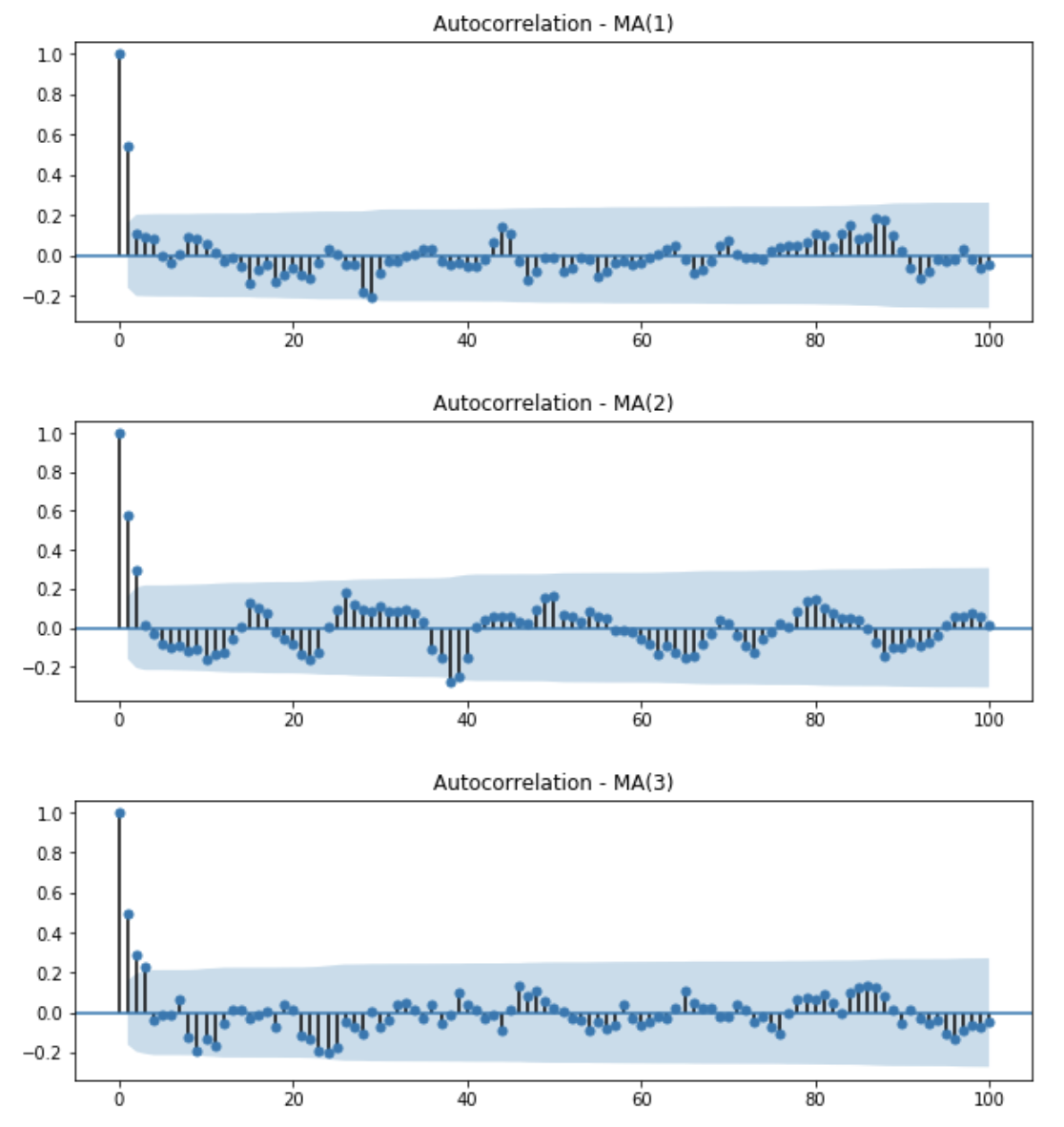
MA(q)에 대해서는 간단합니다. MA process의 정의에 따라, MA(q)는 현재 시점의 데이터 \(X_t\)가 이전 q개의 noise로만 표현되기 때문에 q 이전의 데이터들과는 무관합니다. MA(q)의 ACF는 아래와 같이 q개의 유의미한 spike를 갖고 이후 값들은 모두 0에 가깝습니다(negligible)
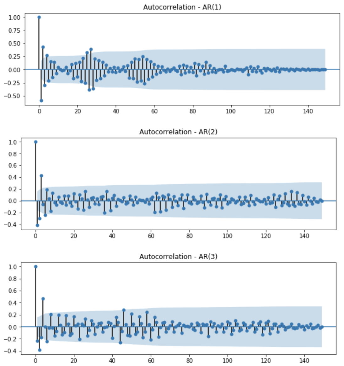
반면 AR(p)는 ACF만으로 p를 결정하기가 어렵습니다. AR process의 ACF는 lag가 증가할수록 decay한 모습을 보일뿐, p에 대한 힌트를 주지 못하기 때문입니다. 다음에서는 주어진 데이터로부터 어떻게 AR(p)모델의 order를 결정할 수 있는지 알아보도록 하겠습니다.
Particial ACF
범죄(crime) 발생 수 와 교회의 수(church)의 상관계수는 양의 상관관계를 갖고 있다고 합니다. 정말로 범죄가 많은 지역에 교회의 수가 많고, 또는 교회의 수가 많은 지역에 범죄가 발생할 가능성도 높은 걸까요? 아닙니다. 이는 두 요인과 관련있는 다른 요인, 인구(population)에 대한 요인을 고려하지 못했기때문에 발생하는 잘못된 결과 해석입니다. 이처럼 두 변수 사이에 수치적 관계가 있는지 또는 어느 정도로 관련이 있는지를 찾을 때, 두 변수와 관련된 다른 변수가있을 경우 해당 상관 계수를 사용하면 잘못된 결과를 얻을 수 있습니다. 이런 경우, 부분 상관 계수(partical correlation)를 계산하여 혼동되는 변수를 제어할 수 있습니다. 범죄 발생 수(X)와 교회의 수(Y)를 각 각 인구(Z)를 독립변수로 하여 회귀 모형을 구한후, 두 회귀 모형의 residual 항만 사용하여 correlation을 구하는 것이 partial correlation입니다.
\[Let \ X = number \ of \ crime, Y = number \ of \ church, Z = population \\ \begin{align} X &= w_X Z + e_{X} \\ Y & = w_Y Z + e_{Y} \\ \\ \rho_{XY \cdot Z} & = \frac{\rho_{XY}-\rho_{XZ}\rho_{YZ}}{\sqrt{1-\rho_{XZ}^2} \sqrt{1-\rho_{YZ}^2}} \end{align}\]Partial correlation의 개념을 시계열 데이터에 적용한 것이 Partial Auto-Correlation Function(PACF)입니다.
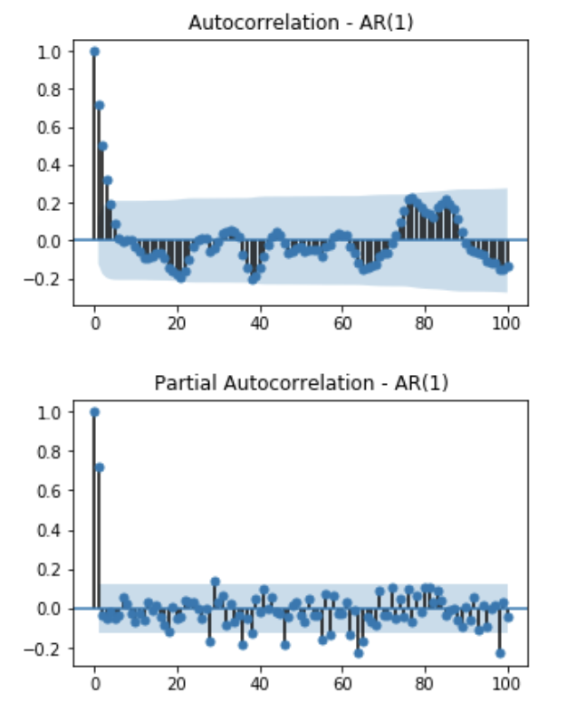
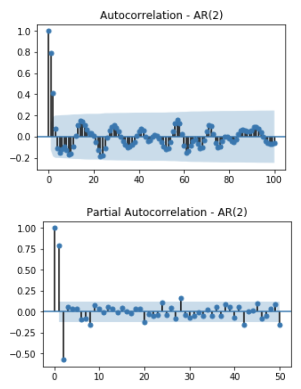
\[\begin{align} \phi_{hh} & = Corr(X_t, X_{t-h} | X_{t-h+1}, X_{t-h+2}, ..., X_{t-1}) \\ & = Corr(X_t - (\alpha_1 X_{t-h+1} + \alpha_2 X_{t-h+2} + ... \alpha_h X_{t-1}), X_{t-h} - (\beta_1 X_{t-h+1} + \beta_2 X_{t-h+2} + ... \beta_h X_{t-1})) \end{align}\]예를 들어 AR(1) 모델의 partial autocorrelation function 은 아래와 같이 계산됩니다.
AR(1) :
\[\begin{align} \phi_{11} &= Corr(X_t, X_{t-1}) = \rho(1) = \phi \\ \phi_{22} &= Corr(X_t, X_{t-2} | X_{t-1}) = Corr(Z_t, Z_{t-1}) = 0 \\ \phi_{33} &= Corr(X_t, X_{t-3} | X_{t-1}, X_{t-2}) = Corr(Z_t, X_{t-2}...) = 0 \end{align}\](참고):
\[\begin{align} \phi_{22} & = Corr(X_t, X_{t-2} | X_{t-1}) \\ & = Corr(X_t - (\alpha X_{t-1}), X_{t-2} - (\beta X_{t-1})) \\ & = Corr(Z_t, Z_{t-1}) & since, \ \alpha = corr(X_t, X_{t-1}) = \phi, \beta = & corr(X_{t-1}, X_{t-2}) = \phi \\ & = 0 \end{align}\]일반적으로 \(\phi_{hh}\)는 위의 메트릭스 형태의 Yule-Walker equation의 마지막 컴포턴트와 같습니다.
\[\begin{bmatrix} \rho(1)\\ \rho(2)\\ \rho(3)\\ \vdots \\ \rho(h-1)\\\rho(h) \end{bmatrix} = \begin{bmatrix} 1 & \rho(1) & \rho(2) & \cdots & \rho(h-1) \\ \rho(1) & 1 & \rho(1) & \cdots & \rho(h-2) \\ \rho(2) & \rho(1) & 1 & \cdots & \rho(h-3) \\ & & \vdots & & \\ \rho(h-2) & \rho(h-3) & \rho(h-4) & \cdots & \rho(1) \\ \rho(h-1) & \rho(h-2) & \rho(h-3) & \cdots & 1 \\ \end{bmatrix} \begin{bmatrix} \phi_{h1}\\ \phi_{h2}\\ \phi_{h3}\\ \vdots \\ \phi_{h(h-1)}\\\phi_{hh} \end{bmatrix}\]AR(2)의 예시와 같이 주어진 데이터가 AR(p) process를 따를경우 PACF의 형태는 lag가 p일때까지는 constant 값을 갖고, 이후의 값은 모두 0에 가까운 값이 됩니다.
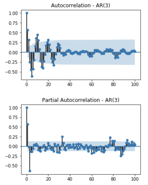
지금까지 알아본 것을 요약하여, 시계열 데이터가 주어졌을때 모델과 모델의 order를 결정하는 방법은 아래와 같습니다.
| AR(p) | MA(q) | ARMA(p, q) | |
|---|---|---|---|
| ACF | tails off | cuts off after lag q | tails off |
| PACF | cuts off after lag p | tails off | tails off |
Reference
[1] Introduction to Time Series and Forecasting, Peter J. Brockwell, Richard A. Davis,
[2] Statsmodel’s Documentation
Comments