Deep Spatio-Temporal Residual Networks for Citywide Crowd Flows Prediction

Junbo Zhang, Yu Zheng, Dekang Qi (Microsoft Research) 2017

Keras implementation : https://github.com/lucktroy/DeepST

Introduction

• Forecating the flow of crowds

• In this paper, we predict two types fo crowd flows : inflow and outflow

• Inflow and outflow of crowds are affected by the following
  • Spatial dependencies
  • Temporal dependencies
  • External influence : such as weather, events
• Contributions
  • ST-ResNet employs convolution-based residual networks to model nearby and distance spatial dependencies between any two regions
  • three categories of temporal properties : temporal closeness, period, and trend. ST-ResNet use three residual netowrks to model these, respectively
  • ST-ResNet dynamically aggregates the output of the three aforementioned networks.

Formulation of Crowd Flows Problem

• Region : we partition a city into an I*J grid map
• Inflow/outflow : Let P be a collection of trajectories at the t^th time interval. For a grid (i, j) that lies at the i^th row and j^th column, the inflow and outflow of the crowds at the tiem interval t are defined respectively as \(x_t^{in, i, j} = \sum_{T_r \in P} |{k > 1 |g_{k-1} \notin (i, j) \land g_k \in (i, j)}| \\ x_t^{out, i, j} = \sum_{T_r \in P} |{k \ge 1 |g_{k-1} \in (i, j) \land g_{k+1} \notin (i, j)}|\) where
  • \(T_r : g_1 \to g_2 \to ... \to g_{\left\vert T_r \right\vert}\) is a trajectory in P
  • \(g_k\) is the geospatial coordinate
  • \(g_k \in (i, j)\) means the point \(g_k\) lies within grid (i, j), and vice versa
  • \(\left\vert \cdot \right\vert\) denotes the cardinality of a set

Deep Spatio-Temporal Residual Networks

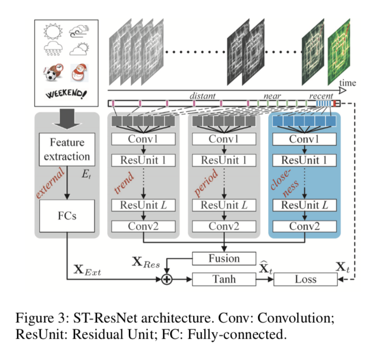
• comprised of four major components modeling temporal closeness, period, trend, and external influence, respectively.

• First, we turn inflow and outflow throughout a city at each time interval into a 2-channel image-like matrix.

• Then, we divide the time axis into three fragments, denoting recent time, near history and distant history. The 2-channel flow matrics of intervals in each time fragment are the fed into the first three components seperately to model the aforementioned three temporal properties: closeness, period, and trend
  • three components share the same network structure(Regisudal Unit sequence)
  • The output of the three components are fused as \(X_{Res}\) based on parameter metrics, which assign different weights to the results of different components in different regions.

• In the external component, we manually extract some feature form external datasets, such as weather conditions and events, feeding them into a two-layer fully-connected neural network.

• \(X_{Res}\) and \(X_{Ext}\) are integrated together. Then, the final output is mapped into [-1, 1] using Tanh function.

Structures of the First Three Components

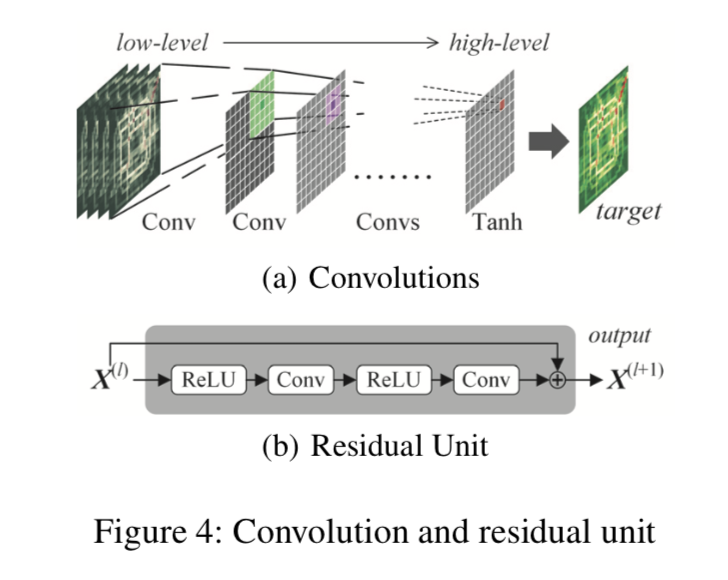
• Do not user subsampling, but only convolutions
• closeness component
  • \([X_{t-l_c}, X_{t-l_c-1}, ..., X_{t-1}]\) : concatnate them along with the first axis
  • \(X_c^{(0)} \in R^{2l_c \times I \times J}\) is followed by conv1
  • Residual Unit : stack \(L\) residual units to capture very large citywide dependencies
  • Residual Unit combinations fo “ReLu + Convolution” and “BatchNormalization” is added before ReLu.
  • On top of the \(L^{th}\) residual unit, we append a convolutional layer conv2
  • output of the closeness componet is \(X_c^{(L+2)}\)

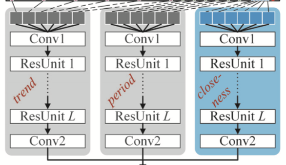
• period component
  • Assume that there are \(l_p\) time intervals from the period fragment and the period is \(p\) ;\([X_{t-l_p \cdot p}, X_{t-(l_p-1) \cdot p}, ..., X_{t-p}]\)
  • output : \(X_p^{(L+2)}\)
  • in implementation, p is equal to one-day (daily periodicity)
• trend component
  • \(l_q\) is the length of the trend dependent sequence and q is the trend span
  • input : \([X_{t-l_q \cdot q}, X_{t-(l_q-1) \cdot q}, ..., X_{t-q}]\)
  • output : \(X_q^{(L+2)}\)
  • in implementation, q is equal to one-week(week trend)

The Structure of the External Component

• mainly consider weather, holiday event, and metadata(DayOfWeek, Weekday/Weekend)

• stack two fully-connected layers upon \(E_t\)

  • first layer : embedding layer
  • second layer : to map low to high dimensions that have the same shape with \(X_t\)

Fusion

• flows of two regions are all affected by closeness, period, and trend, but the degrees of influence may be very different ; parametric-matrix-based fusion

\[X_{Res} = W_c \circ X_c^{L+2} + W_p \circ X_p^{L+2} + W_q \circ X_q^{L+2}\]

• \(\circ\) is Hadamard product (i.e., element-wise multiplication)

• \(W_c, W_p, W_q\) are learnable parameters

• fusing the external component

\[\hat{X_t} = tanh(X_{Res} + X_{Ext})\]

• objectives : minimizing mean squared error between the predicted flow matrix and the true flow matrix.

Experiments

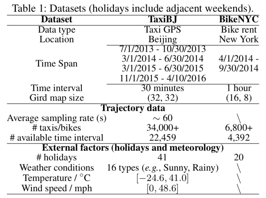
• Datasets

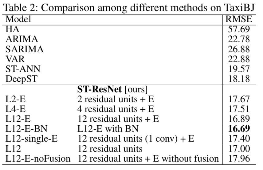
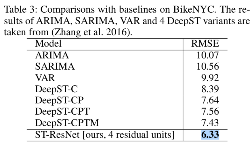
• Baselines
  • HA : historical data (previous week, same time)
  • ARIMA, SARIMA, VAR
  • ST-ANN : It first extracts spatial (nearby 8 regions’ values) and temporal (8 previous time intervals) features, then fed into an artificial neural network.
  • DeepST : (Zhang et al. 2016)
• Preprocessing
  • min-max normalization : [-1, 1] (tanh)
  • one-hot encoding for external data
• Result