
클러스터링을 평가하는 척도 - Mutual Information
클러스터링은 주어진 데이터에 대한 명시적인 정보가 많지 않을 때 유용하게 쓸수있는 머신러닝 기법 중 하나입니다. 다양한 사용자 정보를 이용해 몇가지 고객군으로 분류하여 고객군별 맞춤 전략을 도출한다던지, 유사한 상품(동영상, 음원까지도)군의 속성을 분석하여 의미있는 인사이트를 도출하는 것에 활용됩니다.
클러스터링 알고리즘 측면에서는 전통적인 Hierarchical clustering, K-means clustering 등이 비교적 쉽게 사용되고 있고, 최근에는 딥러닝 기반의 클러스터링 알고리즘이 다양하게 시도되고 있습니다.
여러가지 논문이나 자료들을 찾아보면 클러스터링 결과를 평가하는 방법이 잘 와닿지 않는 경우가 많습니다. 이 포스팅에서는 클러스터링 결과를 평가하는 지표 중 하나인 Mutual Information에 대해 소개하고자 합니다.
클러스터링 결과를 평가하는 방식은 크게 2가지 형태가 있습니다.
- supervised, which uses a ground truth class values for each sample.
- 지도 방식으로 실제 데이터의 클래스가 존재할때입니다.
- 이미 알려진 벤치마크 데이터셋을 이용해 실제 데이터의 라벨링(ground truth)과 클러스터링 결과를 방식입니다.
- unsupervised, which does not and measures the ‘quality’ of the model itself.
- 비지도 방식으로 모델 자체만 이용하여 평가하는 방식입니다.
- 도메인 지식을 사용하거나, 클러스터 내의 분산과 클러스터 간의 거리(SSE;sum of the squared error)등을 고려하여 평가할 수 있습니다.
Mutual Information
Mutual Information은 정보학이나 확률론에서 두 확률 변수간의 상호 의존도를 나타내는 지표입니다. 확률변수 X와 Y가 존재할때, X를 통해서 Y에 대해서 정보(shannons처럼 단위, 일반적으로는 bits)를 얼마나 얻을수 있는가를 의미하는 것으로 결합확률분포 P(X, Y)와 각 변수의 marginal distribution의 곱 P(X)*P(Y)이 얼마나 유사한가로 측정됩니다.
정의
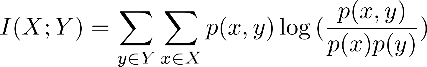
두 개의 이산 확률변수 X와 Y의 Mutual inforamtions는 다음과 정의할 수 있습니다.
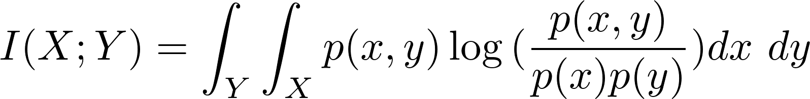
연속 확률 변수의 경우에는 다음과 같습니다.
- X와 Y가 서로 독립적이라면 p(x, y) = p(x) * p(y)가 되어 Mutual Information은 0이 됩니다.
-
또한 X와 Y에 대한 Mutual Information은 p(x, y)와 p(x)*p(y)의 KL divergence와 같습니다.

-
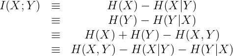
엔트로피 관점에서 Mutual Information은 각 변수가 가진 엔트로피에서 조건부 엔트로피를 뺀 값과 같습니다.
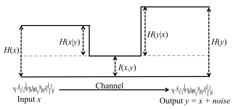
Fig. 엔트로피 다이어그램
클러스터링 평가 지표로서 Mutual information
Mutual Information을 클러스터링 결과를 평가하는 지표로 사용하는 경우는 아래와 같이 정의됩니다. 두가지 클러스터링 할당 결과인 U와 V에 대해서 클러스터에 할당된 확률을 이용합니다.
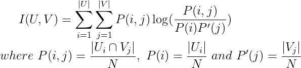
하지만 위의 정의를 그대로 사용할 경우 몇가지 문제점이 있고, 이를 보완하기 위해 Normalized MI와 Adjusted MI 등을 주로 사용합니다.
- 단순히 클러스터의 수가 많을 수록 더 큰 값을 갖게 되는 경향이 있습니다. U와 V의 각 클러스터 수에 따라 정규화할 필요성이 있습니다.
- 랜덤하게 할당된 경우에도 일정값을 갖게 됩니다. 랜덤하게 할당된 경우는 0에 가까운 값이 되도록 하고, U와 V의 두 할당이 같을 때는 1이 되도록 하는 것이 바람직합니다.
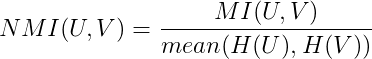
Normalized Mutual Information
Normalized Mutual Information은 Mutual Information 값이 0과 1의 사이 값이 되도록 upper bound 값을 기준으로 정규화한 지표입니다. 이 때 upper bound는 U와 V가 가진 엔트로피(불확실성)의 산술평균값 혹은 기하평균, 최대/최소값 등을 사용할 수 있습니다.
- scikit-learn 패키지를 이용해 NMI를 쉽게 계산할수 있습니다. average_method 파라미터 값을 이용해 정규화 방식을 선택할수 있습니다.
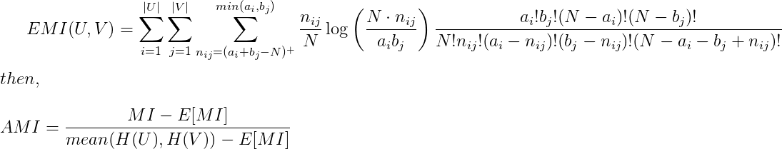
Adjusted Mutual Information
Normalized Mutual information이 0과 1사이의 값을 갖더라도 여전히 클러스터 수가 증가하면 실제 상호의존도와 상관없이 값이 증가하는 경향이 있습니다. 따라서 최근에는 상호의존도의 기대값을 이용해 각 클러스터에 할당될 확률값(chance)으로 조정한 Adjusted Mutual information을 주로 사용합니다. AMI는 두 클러스터링 결과가 랜덤한 경우 0에 가깝고, 할당 결과가 동일한 경우 1이 되도록 합니다.
- scikit-learn 패키지를 이용해 AMI를 쉽게 계산할수 있습니다. average_method 파라미터 값을 이용해 정규화 방식을 선택할수 있습니다.
NMI와 AMI 모두 클러스터 라벨의 절대값과는 무관합니다. 클러스터 라벨이 permutation되더라도 값은 변하지 않습니다.
또한 symmetric하기 때문에 U와 V의 순서를 바꿔도 값은 동일합니다. 데이터의 실제 클래스(groud truth)를 모르더라도 두가지 서로 다른 클러스터링 알고리즘을 비교하는데 유용합니다.
Fashin MNIST를 이용한 K-means Clustering 결과 분석
Keras의 dataset api를 이용해 fashion mnist 데이터를 불러왔습니다. fashion mnist 데이터는 총 10개의 클래스로 이루어져있습니다.
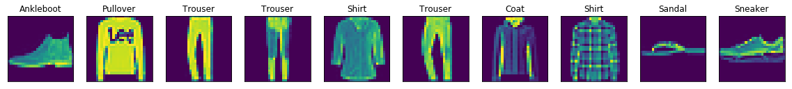
Fig. fashion mnist samples
fashion mnist는 train 데이터 기준으로 클래스별 6000개의 샘플이 있지만, 여기서는 편의상 클래스별로 1000개씩 샘플을 뽑아 K-means 클러스터링을 수행하였습니다.
클러스터링 결과 y_pred와 실제 클래스 라벨인 y_true를 이용해 NMI와 AMI를 계산해보았습니다. NMI와 AMI 모두 symmetric한 성질을 가지고 있는 걸 확인할 수 있습니다.
y_pred = KMeans(n_clusters=10, random_state=0).fit_predict(X)

## check symmetric property
print(normalized_mutual_info_score(y_pred, y_true))
## output : 0.5117333108689629
print(normalized_mutual_info_score(y_true, y_pred))
## output : 0.5117333108689628

print(adjusted_mutual_info_score(y_pred, y_true))
## output : 0.49785636941083883
print(adjusted_mutual_info_score(y_true, y_pred))
## output : 0.49785636941083883
클러스터링 수를 2부터 20까지 증가시키면서 MI, NMI, AMI를 계산해보았습니다. 클러스터 수가 많아질수록 MI 스코어는 0.3 ~ 1.4까지 지속적으로 증가하게 됩니다. 실제 클래스는 10개임에도 불구하고 클러스터 수가 20일 때 가장 높은 값을 갖게 됩니다. 반면에 NMI와 AMI는 클러스터 수가 10 이상에서는 값이 거의 변하지 않는 것을 볼 수 있습니다.
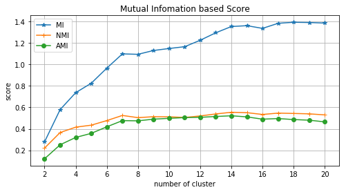
Fig. y_ture vs. K-means : 클러스터 수에 따른 NMI 및 AMI 스코어 변화
그렇다면 k-means 클러스터링이 데이터를 랜덤하게 클러스터링 한것보다 더 나은 것일까요? 10000개의 데이터를 랜덤하게 n개의 클러스터로 할당한 결과(y_random)와 실제 클래스(y_true)의 MI, NMI, AMI를 계산해보았습니다.
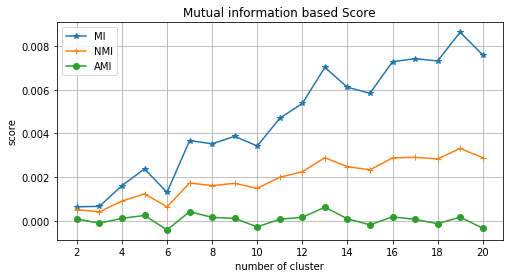 Fig. y_ture vs. random assignment : 클러스터 수에 다른 NMI 및 AMI 스코어 변화
이전 그림과 달리 y-axis의 스케일이 매우 작아진 것이 보이시나요? 3가지 지표 모두 0에 가까운 값을 갖습니다. 또한 (미세하지만) NMI와 MI는 클러스터 수가 증가할 수록 증가하는 경향이 보이지만, AMI는 클러스터 수와 상관없이 0에 아주 가까운 값을 갖습니다.
Appendix. 전체 코드
from keras.datasets import fashion_mnist
from sklearn.cluster import KMeans
from sklearn.manifold import TSNE
import matplotlib.pyplot as plt
import numpy as np
import collections
from sklearn.metrics import adjusted_mutual_info_score, normalized_mutual_info_score, mutual_info_score

%matplotlib inline

class_labels = {0:'T-shirt/top', 1: 'Trouser', 2:'Pullover', 3: 'Dress', 4: 'Coat', \
 5:'Sandal', 6: 'Shirt', 7:'Sneaker', 8:'Bag',9:'Ankleboot'}

(x_train, y_train), (x_test, y_test) = fashion_mnist.load_data()

n = 10
plt.figure(figsize=(20, 4))
for i in range(n):
    # display original
    ax = plt.subplot(2, n, i + 1)
    plt.imshow(x_test[i].reshape(28, 28))
    plt.title(class_labels[y_test[i]])
    ax.get_xaxis().set_visible(False)
    ax.get_yaxis().set_visible(False)
plt.show()

X, y_true = np.empty((0, 28*28)), np.empty((0))
for i in range(10):
    chosen_idx = np.random.choice(np.where(y_train == i)[0], replace=False, size=1000)
    X = np.concatenate((X, x_train[chosen_idx].reshape(-1, 28*28)))
    y_true = np.concatenate((y_true, y_train[chosen_idx]))
y_true_occurence = collections.Counter(y_true)
print('number of samples per class:\n')
for k, v in class_labels.items():
    print(v,' \t: ', y_true_occurence[k])

# number of samples per class:
# T-shirt/top   :  1000
# Trouser       :  1000
# Pullover      :  1000
# Dress         :  1000
# Coat          :  1000
# Sandal        :  1000
# Shirt         :  1000
# Sneaker       :  1000
# Bag           :  1000
# Ankleboot     :  1000

## check symmetric property

y_pred = KMeans(n_clusters=10, random_state=0).fit_predict(X)

print(normalized_mutual_info_score(y_pred, y_true))
## output : 0.5117333108689629
print(normalized_mutual_info_score(y_true, y_pred))
## output : 0.5117333108689628

print(adjusted_mutual_info_score(y_pred, y_true))
## output : 0.49785636941083883
print(adjusted_mutual_info_score(y_true, y_pred))
## output : 0.49785636941083883


## y_true vs. k-means : scores by number of clusters
NMI = []
AMI = []
MI = []
for i in range(2, 21):
    print("number of cluster = ", i)
    y_pred = KMeans(n_clusters=i, random_state=0).fit_predict(X)

    NMI.append(normalized_mutual_info_score(y_true, y_pred))
    AMI.append(adjusted_mutual_info_score(y_true, y_pred))
    MI.append(mutual_info_score(y_true, y_pred))

num_cluster = list(range(2,21))
plt.figure(figsize=(8, 4))
plt.plot(num_cluster, MI, marker='*', label='MI')
plt.plot(num_cluster, NMI, marker='+', label='NMI')
plt.plot(num_cluster, AMI, marker='o', label='AMI')
plt.title('Mutual information based Score')
plt.xlabel('number of cluster')
plt.ylabel('score')
plt.xticks([2, 4, 6, 8, 10, 12, 14, 16, 18, 20])
plt.grid(True)
plt.legend()
plt.show()

## y_true vs. y_random : scores by number of clusters
NMI = []
AMI = []
MI = []
for i in range(2, 21):
    print("number of cluster = ", i)
    y_random = np.random.randint(0, i, 10000)
    y_pred = KMeans(n_clusters=10, random_state=0).fit_predict(X)

    NMI.append(normalized_mutual_info_score(y_pred, y_random))
    AMI.append(adjusted_mutual_info_score(y_pred, y_random))
    MI.append(mutual_info_score(y_pred, y_random))

num_cluster = list(range(2,21))
plt.figure(figsize=(8, 4))
plt.plot(num_cluster, MI, marker='*', label='MI')
plt.plot(num_cluster, NMI, marker='+', label='NMI')
plt.plot(num_cluster, AMI, marker='o', label='AMI')
plt.title('Mutual information based Score')
plt.xlabel('number of cluster')
plt.ylabel('score')
plt.xticks([2, 4, 6, 8, 10, 12, 14, 16, 18, 20])
plt.grid(True)
plt.legend()
plt.show()
Reference
[1] http://scikit-learn.org/stable/modules/classes.html#module-sklearn.metrics.cluster
[2] http://scikit-learn.org/stable/modules/clustering.html#clustering-evaluation
Comments