클러스터링을 평가하는 척도 - Rand Index

클러스터링을 평가하는 척도 - Mutual Information와 이어집니다. 클러스터링 결과를 평가하기 위해 Rand Index 도 자주 쓰입니다. Rand Index는 주어진 N개의 데이터 중에서 2개을 선택해 이 쌍(pair)이 클러스터링 결과 U와 V에서 모두 같은 클러스터에 속하는지, 서로 다른 클러스터에 속하는지를 확인합니다.

Rand Index

n개의 원소로 이루어진 집합 S={o₁, … o_n}와 S를 r개의 부분집합으로 할당한 partition U={U₁, …, U_r}와 S를 s개의 부분집합으로 할당한 partition V={V₁, …, V_r}에 대해서 아래와 같을 때,

a = S의 원소로 이루어진 쌍(pair) 중에서 U와 V에서 모두 동일한 부분집합으로 할당된 쌍의 갯수
b = S의 원소로 이루어진 쌍(pair) 중에서 U와 V에서 모두 다른 부분집합으로 할당된 쌍의 갯수
c = S의 원소로 이루어진 쌍(pair) 중에서 U에서는 동일한 부분집합으로 할당되었지만, V에서는 다른 부분집합으로 할당된 쌍의 갯수
d = S의 원소로 이루어진 쌍(pair) 중에서 U에서는 다른 부분집합으로 할당되었지만, V에서는 동일한 부분집합으로 할당된 쌍의 갯수

Rand Index, RI는 다음과 같이 정의됩니다.

직관적으로 분모는 S에 속하는 n개의 원소 중에서 2개를 뽑는 경우의 수, S의 원소로 가능한 모든 쌍(pair)의 갯수를 의미하고, 분자인 a와 b는 U와 V의 결과가 서로 일치하는 쌍의 갯수를 의미합니다.

클러스터링 평가 지표로서 Rand Index

클러스터링 결과는 n개의 주어진 데이터를 r개 혹은 s개의 부분집합으로 할당하는 것과 같습니다. 즉 위의 정의에서 partition U와 partition V는 두개의 서로 다른 클러스터링 결과에 해당됩니다.

예를 들어, {a, b, c, d, e, f} 총 6개의 데이터가 존재하고 첫번째 클러스터링 알고리즘을 적용한 결과가 U = [1, 1, 2, 2, 3, 3]와 같고, 두번째 클러스터링 알고리즘을 적용한 결과 V = [1, 1, 1, 2, 2, 2]라고 합시다.

6개의 데이터로 가능한 pair는 {a, b}, {a, c}, {a, d}, {a, e}, {a, f}, {b, c}, {b, d}, {b, e}, {b, f}, {c, d}, {c, e}, {c, f}, {d, e}, {d, f}, {e, f}로 총 15개입니다.

그중에서 {a, b}는 U와 v에서 모두 동일한 클러스터에 할당됩니다. (a와 b가 U에서 클러스터1, V에서도 클러스터1에 할당) 마찬가지로 {e, f}도 동일한 클러스터에 할당됩니다. (U에서는 클러스터3에 할당, V에서는 클러스터2에 할당)

반면에 {a, d}는 U와 V에서 모두 다른 클러스터에 할당되는 쌍입니다. (U에서는 a는 클러스터1이고 d는 클러스터2, V에서는 a는 클러스터1이고 d는 클러스터2) {a, e}, {a, f}, {b, d}, {b, e}, {b, f}, {c, e}, {c, f} 도 마찬가지로 서로 다른 클러스터에 할당됩니다.

나머지 쌍 {c, d}, {d, e} 은 U에서는 동일한 클러스터에 할당되었지만, V에서는 다른 클러스터에 할당되거나 그 반대에 해당하는 경우들입니다.

위의 내용을 토대로 최종 Rand Index는 (2+8) / 15 = 0.667이 됩니다.

Rand Index는 항상 0과 1사이의 값을 갖습니다.

두가지 클러스터링 결과인 U와 V가 서로 완전히 일치할 때, Rand Index는 1의 값을 갖습니다. 반대로 어떤 데이터 쌍에 대해서도 일치된 결과를 보이지 않을 경우 0의 값을 갖게 됩니다.

하지만 Rand Index를 그대로 사용하는 경우는 없습니다. 사례를 통해 살펴보겠습니다. 지난번에 살펴보았던 Fashin MNIST를 이용해 데이터를 랜덤으로 할당한 결과(y_random)와 실제 클래스(y_true)의 rand index를 구해보겠습니다.

scikit-learn에는 rand index를 바로 계산하는 api가 없네요.

from keras.datasets import fashion_mnist
import numpy as np

def rand_index(y_true, y_pred):
    n = len(y_true)
    a, b = 0, 0
    for i in range(n):
        for j in range(i+1, n):
            if (y_true[i] == y_true[j]) & (y_pred[i] == y_pred[j]):
                a +=1
            elif (y_true[i] != y_true[j]) & (y_pred[i] != y_pred[j]):
                b +=1
            else:
                pass
    RI = (a + b) / (n*(n-1)/2)
    return RI

_, (X, y_true) = fashion_mnist.load_data()
y_random = np.random.randint(0, 10, 10000)


print(rand_index(y_true, y_random))
## output : 0.8200785478547855

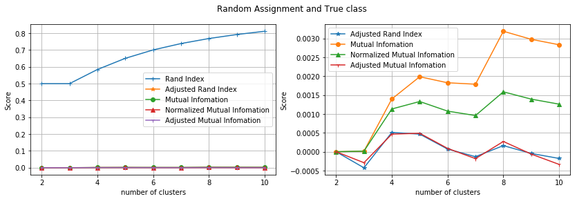
랜덤하게 클래스를 할당했음에도 불구하고 RI가 0.82로 높게 나타납니다. 클러스터의 수가 증가할수록 pair를 이루는 두 데이터가 서로 다른 클러스터에 속할 확률이 높아지기 때문입니다. 이로 인해 클러스터 수가 많아지면 b값이 커질 확률이 크고, rand index도 높은 값을 갖습니다.

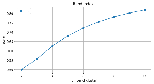Fig. 클러스터 수에 따른 Rand Index 변화

이런건 우리가 원하는게 아니잖아요?

Adjusted Rand Index

따라서 일반적으로 Rand Index를 확률적으로 조정한 Adjusted Rand Index를 사용합니다. contingency table은 U와 V partition을 |U_i ∩ V_i| = n_ij 로 표기하여 요약한 테이블로 아래와 같은 contingency table이 주어질 때, ARI는 다음과 같이 정의 됩니다.

\[\newcommand\T{\Rule{0pt}{1em}{.3em}} \begin{array} {c|lllr|c} U \setminus V & V_1 & V_2 & \cdots & V_s & Sums \\ \hline U_1 & n_{11} & n_{12} & \cdots & n_{1s} & a_1 \\ U_2 & n_{21} & n_{22} & \cdots & n_{2s} & a_2 \\ \vdots & \vdots & \vdots & \cdots & \vdots & \vdots \\ U_r & n_{r1} & n_{r2} & \cdots & n_{rs} & a_r \\ \hline Sums & b_1 & b_2 & \cdots & b_s & \\ \end{array}\]

위와 마찬가지로 Fashin MNIST 데이터를 랜덤으로 할당한 결과(y_random)와 실제 클래스(y_true)를 이용해 Adjusted Rand Index를 구해보겠습니다.

scikit-learn 패키지를 이용해 ARI를 쉽게 계산할수 있습니다.

from keras.datasets import fashion_mnist
from sklearn.metrics import adjusted_rand_score
import numpy as np

_, (X, y_true) = fashion_mnist.load_data()
y_random = np.random.randint(0, 10, 10000)


print(adjusted_rand_score(y_true, y_random))
## output : -0.00016616515609661287

ARI는 0에 가까운 값이 나오는 것을 확인할 수 있습니다. 또한 클러스터 수가 증가하더라도 값이 증가하지 않는 것을 볼수 있습니다.

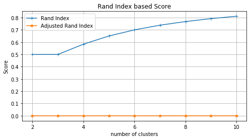
또한 Mutual Information based Score(MI, Normalized MI, Adjusted MI)와도 비교해았습니다. Rand Index를 제외하고 4가지 스코어는 모두 0에 가까운 값이 나타납니다. 랜덤으로 클러스터를 할당한 것과 실제 클래스와의 아무런 상관이 없으니까요. 다만 MI, NMI의 경우 클러스터가 증가할 수록 값이 증가하는 경향이 있지만, 확률적으로 조정된 AMI와 ARI는 클러스터 수에 상관없이 0에 가까운 값을 유지한다는 경향이 있다는 것을 알수 있습니다.

Adjusted Mutual Information 혹은 Adjusted Rand Index를 사용하세요. paper works에서 자주 사용하는 지표는 NMI이니 참고하세요.

Appendix. 전체 코드

from keras.datasets import fashion_mnist
from sklearn.cluster import KMeans
from sklearn.manifold import TSNE
import matplotlib.pyplot as plt
import numpy as np
import collections
from sklearn.metrics import adjusted_mutual_info_score, normalized_mutual_info_score, \
mutual_info_score, adjusted_rand_score

%matplotlib inline

class_labels = {0:'T-shirt/top', 1: 'Trouser', 2:'Pullover', 3: 'Dress', 4: 'Coat', \
 5:'Sandal', 6: 'Shirt', 7:'Sneaker', 8:'Bag',9:'Ankleboot'}

_, (X_all, y_all) = fashion_mnist.load_data()

def rand_index(y_true, y_pred):
    n = len(y_true)
    a, b = 0, 0
    for i in range(n):
        for j in range(i+1, n):
            if (y_true[i] == y_true[j]) & (y_pred[i] == y_pred[j]):
                a +=1
            elif (y_true[i] != y_true[j]) & (y_pred[i] != y_pred[j]):
                b +=1
            else:
                pass
    RI = (a + b) / (n*(n-1)/2)
    return RI

RI = []
ARI = []
AMI = []
NMI = []
MI = []
for i in range(2, 11):
    X, y_true = np.empty((0, 28*28)), np.empty((0))
    for j in range(i):
        chosen_idx = np.where(y_all == j)[0]
        X = np.concatenate((X, X_all[chosen_idx].reshape(-1, 28*28)))
        y_true = np.concatenate((y_true, y_all[chosen_idx]))
    y_random = np.random.randint(0, j, len(y_true))
    ARI.append(adjusted_rand_score(y_true, y_random))
    RI.append(rand_index(y_true, y_random))
    MI.append(mutual_info_score(y_true, y_random))
    NMI.append(normalized_mutual_info_score(y_true, y_random))
    AMI.append(adjusted_mutual_info_score(y_true, y_random))

plt.figure(figsize=(14, 4))
plt.subplot(121)
plt.plot(range(2,11), RI, marker='+', label='Rand Index')
plt.plot(range(2,11), ARI, marker='*', label='Adjusted Rand Index')
plt.plot(range(2,11), MI, marker='o', label='Mutual Infomation')
plt.plot(range(2,11), NMI, marker='^', label='Normalized Mutual Infomation')
plt.plot(range(2,11), AMI, marker='1', label='Adjusted Mutual Infomation')
plt.legend()
plt.ylabel('Score')
plt.xlabel('number of clusters')
plt.xticks([2, 4, 6, 8, 10])
plt.grid()
plt.subplot(122)
plt.plot(range(2,11), ARI, marker='*', label='Adjusted Rand Index')
plt.plot(range(2,11), MI, marker='o', label='Mutual Infomation')
plt.plot(range(2,11), NMI, marker='^', label='Normalized Mutual Infomation')
plt.plot(range(2,11), AMI, marker='1', label='Adjusted Mutual Infomation')
plt.legend()
plt.ylabel('Score')
plt.xlabel('number of clusters')
plt.xticks([2, 4, 6, 8, 10])
plt.grid()
plt.suptitle('Random Assignment and True class')
plt.show()

Reference

[1] https://en.wikipedia.org/wiki/Rand_index

[2] http://scikit-learn.org/stable/modules/generated/sklearn.metrics.adjusted_rand_score.html#sklearn.metrics.adjusted_rand_score

[3] https://davetang.org/muse/2017/09/28/rand-index-versus-adjusted-rand-index/

Twitter Facebook Google+ LinkedIn

yjucho

클러스터링을 평가하는 척도 - Rand Index

Rand Index

클러스터링 평가 지표로서 Rand Index

Adjusted Rand Index

Reference

Comments