Dynamic Time Warping(DTW)

두 시계열 데이터간의 유사도를 어떻게 계산할 수 있을까? 두 시계열이 동일한 길이의 시퀀스라면 단순히 상관계수를 구하는 것이 가능하지만, 현실 세계의 시계열 데이터는 그렇지 않은 경우가 많습니다. 예를 들어 아래와 같은 두 시계열 데이터를 살펴보겠습니다.

import matplotlib.pyplot as plt

ts1 = [1, 5, 3, 4, 7, 6]
ts2 = [0, 2, 6, 3, 5, 6, 8, 5]

plt.figure(figsize=(15,5))
plt.subplot(121)
plt.title('Time series 1')
plt.plot(ts1)
plt.grid(True)
plt.subplot(122)
plt.title('Time series 2')
plt.plot(ts2)
plt.grid(True)
plt.show()

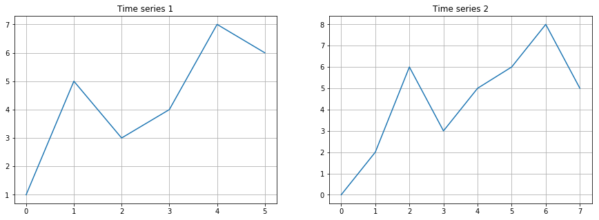
육안으로 보기엔 두 시계열 모두 두 개의 peak를 가지고 있고 전체적으로 우상향하는 모습이 매우 유사해보입니다. 두 시계열 간의 상관계수를 구해보도록 하겠습니다. 어랏, 두 데이터의 길이가 다르기 때문에 바로 계산되지 않네요.

np.corrcoef(ts1, ts2)
## ValueError: all the input array dimensions except for the concatenation axis must match exactly

유사도를 측정하기 위한 가장 간단한 방법은 상대적으로 길이가 짧은 시계열1 데이터를 interpolation하여 길이를 동일하게 맞춘 후, np.corrcoef를 사용하여 상관계수를 계산하는 것입니다.

import numpy as np

len_ts1 = len(ts1)
len_ts2 = len(ts2)
interval = len_ts2 / float(len_ts1)
interp_ind = np.arange(0, len_ts2, interval)
ts1_interp = np.interp(np.arange(0,len_ts2, 1), interp_ind, ts1)
plt.figure(figsize=(15,5))
plt.subplot(121)
plt.title('Time series 1')
plt.plot(ts1)
plt.grid(True)
plt.subplot(122)
plt.title('Comparison : ts1_interp vs. ts2')
plt.plot(ts1_interp)
plt.plot(ts2)
plt.legend(['Time series 1 - interpolation', 'Time series 2'])
plt.grid(True)
plt.show()

## correlation coefficent
np.corrcoef(ts1_interp, ts2)
#### output
# array([[ 1.        ,  0.85206492],
#        [ 0.85206492,  1.        ]])

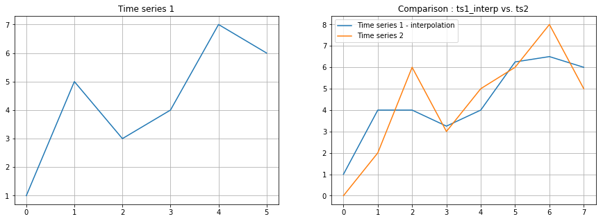
단순히 선형 보간(linear interpolation) 방법은 기존의 시계열 데이터1이 가지고 있는 모습을 꽤 왜곡시킨는 결과를 낳습니다. 2개의 spike형태의 peak가 사라진 것을 볼 수 있습니다. 실제로 단순히 데이터 포인트를 늘려서 대응방식으로 비교하는 것은 합리적이지 못한 경우가 많습니다.

이렇게 길이가 서로 다른 두 시계열의 유사도를 계산하는 방법으로 DTW(Dynamic Time Warping)를 사용할 수 있습니다. DTW는 시퀀스의 길이를 고려하지 않기 때문에 서로 다른 길이의 시퀀스의 유사도를 바로 계산할 수 있습니다.

In time series analysis, dynamic time warping (DTW) is one of the algorithms for measuring similarity between two temporal sequences, which may vary in speed. For instance, similarities in walking could be detected using DTW, even if one person was walking faster than the other, or if there were accelerations and decelerations during the course of an observation. DTW has been applied to temporal sequences of video, audio, and graphics data — indeed, any data that can be turned into a linear sequence can be analyzed with DTW. A well known application has been automatic speech recognition, to cope with different speaking speeds. Other applications include speaker recognition and online signature recognition. Also it is seen that it can be used in partial shape matching application. - 위키피디아

** 아래는 DTW의 개념을 소개하기 위해 jsideas님의 포스팅를 인용하였습니다.

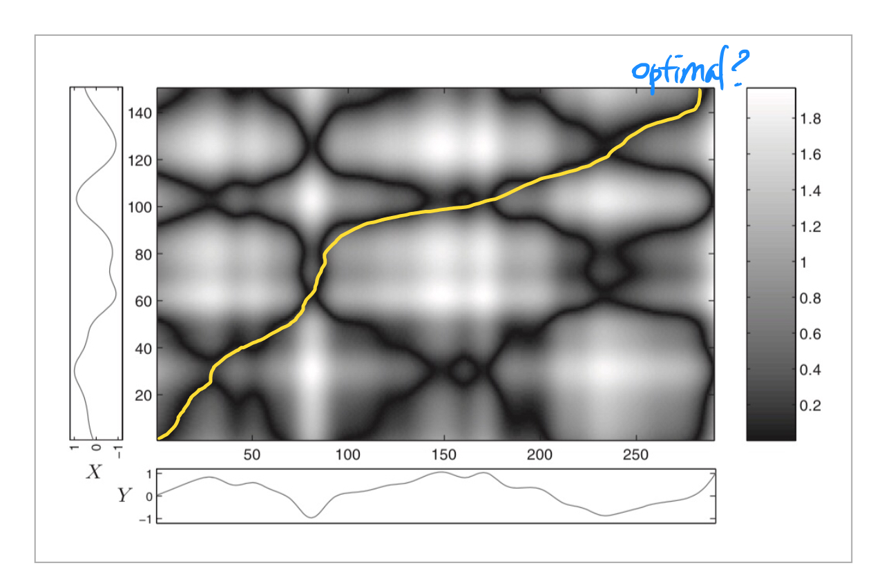
n개의 데이터포인트가 있는 시퀀스 X와 m개의 데이터포인트가 있는 시퀀스 Y가 있다고 하겠습니다. 이 두 시퀀스를 각 각 x축과 y축에 늘어놓고 데이터 포인트간의 거리(예를 들어 유클리디언 거리)를 구하면, 그 값둘은 m\(\times\)n의 매트릭스 형태가 됩니다. 이 매트릭스를 cost matrix라고 하도록 하겠습니다. cost matrix를 heatmap형식으로 표현하면 아래 그림처럼, 두 데이터 포인트간 거리가 짧은 곳은 어둡게, 거리가 먼 곳은 흰색으로 표현됩니다. DTW알고리즘은 저 cost matrix 상의 좌하단에서 우상단까지 가는 최적의 경로를 찾는 문제를 푸는 것입니다.

이 최적화문제의 목적식은 좌하단(0,0)에서 우상단(m, n)을 이동하는데 드는 비용을 최소화하는 것이고, 이때 3가지 제약조건이 존재하게 됩니다.

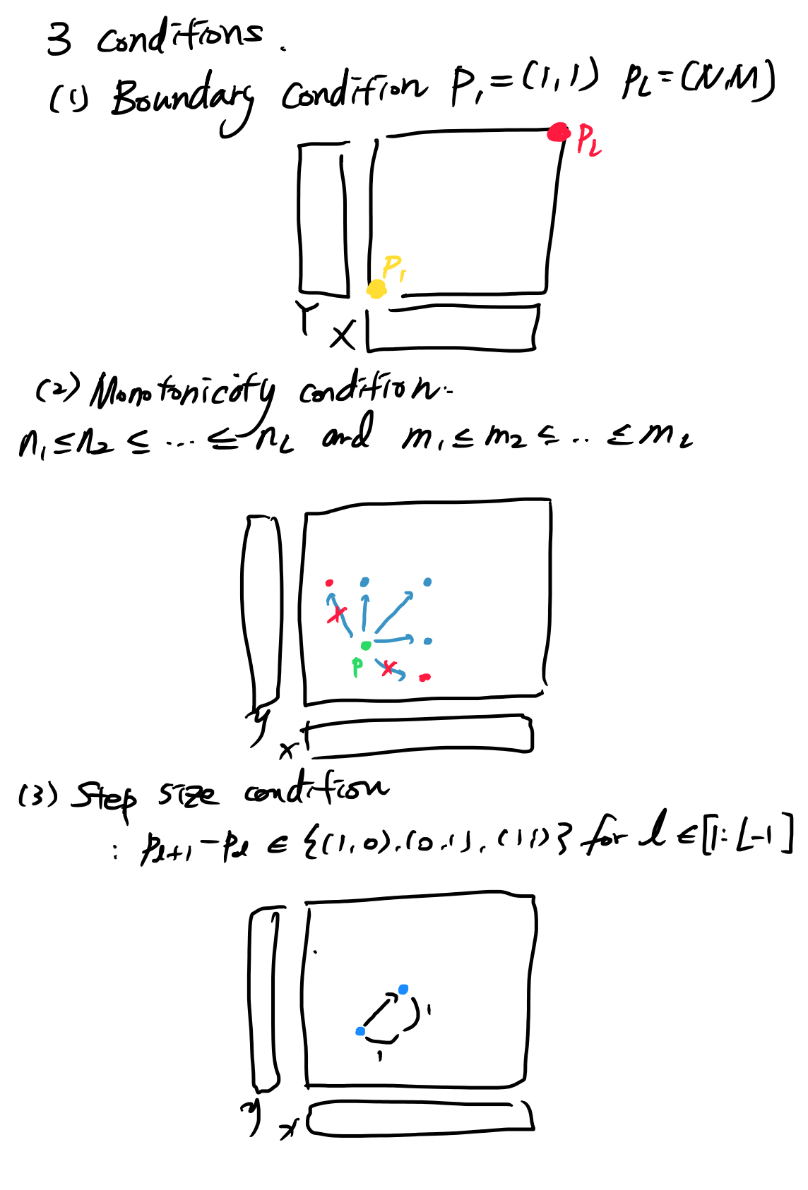
두 시퀀스의 처음과 끝은 같아야 합니다. 즉 무조건 좌하단에서 시작해서 우하단에서 끝나야합니다.
x나 y축, 혹은 그 두 축에서 음의 방향으로 이동하지 않습니다.
이동할때 정해진 스텝사이즈 (예를 들어 오른쪽과 위쪽 한칸씩만 이동가능하다던지..(0,1) or (1,0) or (1,1))만큼 이동가능합니다. 가능한 스텝사이즈를 늘릴수록 더 많은 경우 수를 검색하기 때문에 최적에 가까운 경로를 얻을 수 있지만, 그만큼 계산속도가 느려지게 됩니다.

DTW는 결국 X와 Y를 늘어놓고 X의 특정 데이터포인트가 Y의 어떤 데이터포인트에 가장 적합한지를 판정하는 로직이므로, X와 Y의 길이가 늘어나면 늘어날수록 검색 비용이 늘어나는 단점이 있습니다.

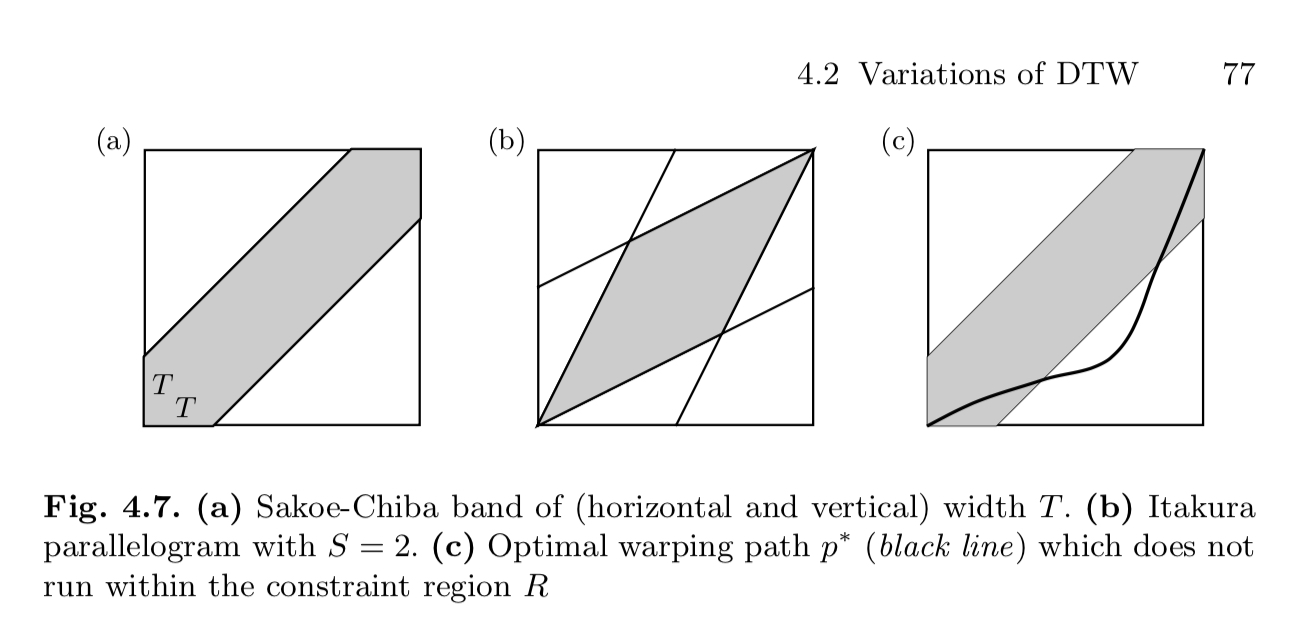
또한 앞서 언급했듯이 최적값을 찾기 위해 검색가능한 스텝사이즈를 늘리면 계산 속도가 느려지게 되고, 반대로 스텝사이즈를 줄이면 전후 경로만 보고 기계적으로 두 시퀀스를 정렬시켜버리는 pathological alignment 문제가 발생할 수 있습니다. 일반적으로 pathological alignment문제를 피하기 위해 Sakoe-Chiba Band와 Itakura Parallelogram방법 등을 사용하기도 합니다.

python에서의 DTW

파이썬에서는 pip 패키지인 dtw를 통해서 별도의 구현없이 DTW알고리즘을 쉽게 이용할 수 있습니다.

https://pypi.org/project/dtw/

github description : https://github.com/pierre-rouanet/dtw

패키지를 설치한 후 아래와 같이 사용할 수 있습니다.

from dtw import dtw
x = np.array(ts1).reshape(-1,1)
y = np.array(ts2).reshape(-1,1)

euclidean_norm = lambda x, y: np.abs(x - y)

d, cost_matrix, acc_cost_matrix, path = dtw(x, y, dist=euclidean_norm)

plt.imshow(acc_cost_matrix.T, origin='lower', cmap='gray', interpolation='nearest')
plt.plot(path[0], path[1], 'w')
plt.show()

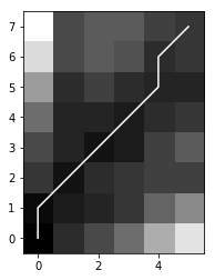
cost matrix와 최적 path는 위 이미지에 표시된것과 같고, 이를 다시 시계열 차트에서 비교하면 아래와 같습니다. dtw를 통해 warping된 시계열데이터1과 시계열데이터2의 상관계수를 구한 결과, 약 0.92로 단순 선형 보간에 의한 상관계수 0.85보다 더 높은 값이 계산되는 것을 볼 수 있습니다.

ts1_dtw = [ts1[p] for p in path[0]]

plt.figure(figsize=(15,5))
plt.subplot(121)
plt.title('Time series 1')
plt.plot(ts1)
plt.grid(True)
plt.subplot(122)
plt.title('Comparison : ts1_dtw vs. ts2')
plt.plot(ts1_dtw)
plt.plot(ts2)
plt.legend(['Time series 1 - Warping', 'Time series 2'])
plt.grid(True)
plt.show()

np.corrcoef(ts1_dtw, ts2)
#### output
# array([[ 1.        ,  0.92247328],
#        [ 0.92247328,  1.        ]])