
시계열 분석 part4 - VAR
지금까지는 시계열 데이터가 univariate일 경우를 모델링하는 방법을 알아보았습니다. 이번 포스팅에서는 여러개의 시계열 데이터가 존재할 경우, 즉 multivariate 모델인 Vector AutoRegression (VAR) Model을 알아보도록 하겠습니다.
Bivariate time series에 대해서 알아보도록 하겠습니다. Bivariate time series는 2차원의 벡터 시리즈로 표현됩니다. \((X_{t1}, X_{t2})’\) at time t ( t= 1, 2, 3, …) 와 같이 표현하도록 하겠습니다. 두 컴포넌트 \(\{X_{t1}\}\)와 \(\{X_{t2}\}\)를 각 각 독립적인 univariate time series로 분석할 수 있지만, 만약 두 컴포넌트사이에 dependency가 존재할 경우 이를 고려해서 모델링하는 것이 더 바람직합니다.
랜덤 벡터 \(\mathbf{X_t} =(X_{t1}, X_{t2})\)’에 대해서 평균벡터와 공분산 메트릭스는 \(\mu_t\)와 \(\Gamma(t+h, t)\)와 같이 정의됩니다.
\[\mu_t := EX_t = \begin{bmatrix} EX_{t1} \\ EX_{t2} \end{bmatrix}\] \[\Gamma(t+h, t) := Cov(\mathbf{X_{t+h}, X_t}) = \begin{bmatrix} Cov(X_{t+h,1}, X_{t1}) & Cov(X_{t+h,1}, X_{t2}) \\ Cov(X_{t+h,2}, X_{t1}) & Cov(X_{t+h,2}, X_{t2}) \end{bmatrix}\]또한 univariate와 마찬가지로 \(\mu_t\)와 \(\Gamma(t+h, t)\)가 모두 t와 독립적일 때, (weakly) stationary하다고 정의합니다. 이 때의 공분산 메트릭스는 \(\Gamma(h)\)로 표기하고, 메트릭스의 diagonal은 각 각 univariate series인 \(\{X_{t1}\}\)와 \(\{X_{t2}\}\)의 Auto-Covariance Function와 같습니다. 반면 off-diagonal elements는 \(X_{t+h, i}\)와 \(X_{t, i}\), \(i \ne j\)의 covariances를 나타냅니다. 이 때, \(\gamma_{12}(h) = \gamma_{21}(-h)\) 의 특성이 있습니다.
\[\Gamma(h) := Cov(\mathbf{X_{t+h}, X_t}) = \begin{bmatrix} \gamma_{11}(h) & \gamma_{12}(h) \\ \gamma_{21}(h) & \gamma_{22}(h) \end{bmatrix} \\\]\(\mu\) vector와 \(\Gamma(h)\), \(\rho_{ij}(h)\)의 estimator는 다음과 같습니다.
\[\bar{\mathbf{X_n}} = \frac{1}{n} \sum_{t=1}^n\mathbf{X_t}\] \[\begin{align} \hat\Gamma(h) & = n^{-1} \sum_{t=1}^{n-h} \left( \mathbf{X_{t+h}} - \bar{\mathbf{X_n}} \right) \left( \mathbf{X_{t}} - \bar{\mathbf{X_n}} \right) \ \ \ \ \ \ \ & for \ 0 \le h \le n-1 \\ & = \hat\Gamma(-h)'\ \ \ \ \ \ \ & for \ -n+1 \le h \le 0 \\ \end{align}\]correlation between \(X_{t+h,i}\) and \(X_{t,j}\)
\[\hat{\rho_{ij}}(h) = \hat{\gamma_{ij}}(h) (\hat{\gamma_{ii}}(0)\hat{\gamma_{jj}}(0))^{-1/2}\]이를 m개의 다변량 시계열 데이터로 확대하면 다음과 같습니다.
\[\mathbf{X_t} :=\begin{bmatrix} X_{t1} \\ \vdots \\ X_{tm} \end{bmatrix}\] \[\mu_t := EX_t = \begin{bmatrix} \mu_{t1} \\ \vdots \\ \mu_{tm} \end{bmatrix}\] \[\Gamma(t+h, t) := \begin{bmatrix} \gamma_{11}(t+h, t) & \cdots & \gamma_{1m}(t+h, t) \\ \vdots & \vdots & \vdots \\ \gamma_{m1}(t+h, t) & \cdots & \gamma_{mm}(t+h, t) \end{bmatrix} \\ where \ \gamma_{ij}(t+h, t):=Cov(X_{t+h, i}, X_{t, j})\]Definition
The m-variate series \(\{\mathbf{X_t}\}\) is (weakly) stationary if
(1) \(\mu_X(t)\) is independent of t, and
(2) \(\Gamma_X(t+h, t)\) is independent of t for each h.
이 때 \(\gamma_{ij}(\cdot)\), \(i \ne j\) 는 서로 다른 두 시리즈 \(\{X_{ti}\}\)와 \(\{X_{tj}\}\) 의 cross-covariance라고 부릅니다. 일반적으로 \(\gamma_{ij}(\cdot)\)는 \(\gamma_{ji}(\cdot)\)와 같지 않기 때문에 주의하셔야합니다.
Basic Properties of \(\Gamma(\cdot)\):
(1) \(\Gamma(h) = \Gamma'(h)\) \
(2) \(\left\vert\gamma_{ij}(h)\right\vert \le [\gamma_{ii}(0)\gamma_{jj}(0)]^{1/2}\), i,j=1,…,m
(3) \(\gamma_{ii}(\cdot)\) is an autocovariance function, i = 1,…,m
(4) \(\rho_{ii}(0) = 1\) for all i
Univariate에서 살펴본 white noise 역시 아래와 같이 다변량 정규분포를 따르는 벡터로 정의됩니다.
Definition
The m-variate series \(\{Z_t\}\) is called white noise with mean 0 and covariance matrix \(\Sigma\), written
\(\{Z_t\} \sim WN(\mathbf{0}, \Sigma)\),
if \(\{Z_t\}\) is stationary with mean vector \(\mathbf{0}\) and covariance matrix function
\(\begin{align} \Gamma(h) & = \Sigma, \ \ if \ h = 0 \\ & = 0, \ \ \ \ otherwise. \end{align}\)
White noise의 선형조합으로 표현되는 m-variate series \(\{X_t\}\)를 linear process로 부르며, MA(\(\infty\)) 프로세스는 j가 0보다 작은 경우에는 \(C_j=0\)인 linear process에 해당합니다.
Definition
The m-variate series \(\{X_t\}\) is a linear process if it has the representation
\(\mathbf{X_t} = \sum_{j=-\infty}^\infty C_j \mathbf{Z_{t-j}}, \ \ \ \ \ \{\mathbf{Z_{t-j}}\} \sim WN(\mathbf{0}, \mathbf{\Sigma})\),
where \(\{C_j\}\) is a sequence of m X m matrics whose components are absolutely summable.
또한 causality를 만족하는 모든 ARMA(p, q) 프로세스는 MA(\(\infty\)) 프로세스로 변환할 수 있으며, invertibiliy를 만족하는 모든 ARMA(p, q) 프로세스는 AR(\(\infty\)) 프로세스로 변환할 수 있습니다. causality 조건을 만족하면 항상 stationary하고, stationary ARMA(p, q) process는 항상 causality를 만족합니다.
Causality
An ARMA(p, q) process \(\{X_t\}\) is causal, or a causal function of \(\{Z_t\}\), if there exist matrices \(\{\Psi_t\}\) with absolutely summable components such that
\(X_t = \sum_{j=0}^{\infty}\Psi_jZ_{t-j}\) for all t.
Causality is equivalent to the condition
\(det\Phi(z) \ne 0\) for all \(z \in \mathbb{C}\) such that \(\vert z \vert \le 1\)
Causality 조건을 다시 보면 1보다 작은 모든 z에 대해서 \(\Phi(z)\)의 determinant는 0이 아니여야합니다. 이는 \(\Phi(z)\)의 모든 eigenvalue들이 1보다 작아야한다 것과 동일합니다.
Yule-walker equation
Yule-walker equation을 이용해 모델의 파라미터를 추정하는 방법에 대해서 살펴보도록 하겠습니다. 실제로는 소프트웨어를 통해 계산되기 때문에 복잡한 계산을 수행할 필요는 없지만, 원리를 이해하는 것을 목적으로 합니다.
양변에 \(X_{t-h}'\)를 곱해줍니다.
\[X_t X_{t-h}' = \Phi X_{t-1}X_{t-h}' + Z_tX_{t-h}'\]이후 Expectation을 취해줍니다.
\[E[X_t X_{t-h}'] = \Phi E[ X_{t-1}X_{t-h}' ] + E[Z_tX_{t-h}' ]\]\(X_t\)의 평균이 0인 시리즈라고 가정하고, h가 1보다 크거나 같을 때와 h가 0일때로 나눠서 생각해볼수 있습니다. \(\begin{align} \Gamma(h) & = \Phi \Gamma(h-1) + \mathbf{0} \ \ \ \ \ \ for \ h \ge 1 \\ \Gamma(0) & = \Phi \Gamma(-1) + \Sigma_Z \\ & = \Phi \Gamma(1)' + \Sigma_Z \ \ \ \ \ \ for \ h =0 \end{align}\)
h가 1일때와 h가 0일때의 두 식을 연립하여 풀면 \(\Phi\)를 구할수 있습니다. \(\begin{align} \Gamma(1) & = \Phi \Gamma(0) + \mathbf{0} \ \ \ \ \ \ for \ h = 1 \\ \Gamma(0) & = \Phi \Gamma(1) + \Sigma_Z \ \ \ \ \ \ for \ h =0 \end{align}\)
Cointegration
앞선 nonstationary univariate time series에서 \(\nabla = 1-B\)를 이용하여 stationary를 만드는 방법을 이야기한 적 있습니다. 만약 \(\{\nabla^d X_t\}\)가 어떤 양수 d에 대해서 stationary이나, \(\{\nabla^{d-1} X_t\}\)에 대해서는 nonstationary할 때, \(\{X_t\}\) is integrated of order d라고 하며, \(\{X_t\} \sim I(d)\)라고 표기합니다. 마찬가지로 \(\{X_t\}\) 가 k-variate time series일 경우에도, \(\{\nabla^{d} X_t\}\)는 j번째(j=1, …, k) 컴포넌트에 \((1-B)^d\) 오퍼레이터를 적용하여 얻은 시리즈를 의미합니다.
cointegration이라는 개념은 Granger(1981)에서 처음 도입되고, Engle and Granger(1987)가 개발하였습니다. 여기서는 Lukepohl(1993)의 개념을 사용하도록 하겠습니다.
If d is a positive integer, \(\{\nabla^d X_t\}\) is stationary and \(\{\nabla^{d-1} X_t\}\) is nonstationary, the k-dimensional time series \(\{X_t\}\) is integrated of order d (\(\{X_t\} \sim I(d)\)).
The I(d) process \(\{X_t\}\) is said to be cointegrated with cointegration vector \(\alpha\) if \(\alpha\) is a k \(\times\) 1 vector such that \(\{\alpha' X_t\}\) is integrated of order less than d.
example
\[\begin{align} X_t = \sum_{j=1}^t Z_j, & & t =1, 2, ..., \ \ & \{Z_t\} \sim IID(0, \sigma^2) \\ Y_t = X_t + W_t, & & t=1, 2, ..., \ \ & \{W_t\} \sim IID(0, \tau^2) \\ \end{align}\]where \(\{W_t\}\) is independent of \(\{Z_t\}\). Then \(\{(X_t, Y_t)'\}\) is integrated of order 1 and cointegrated with cointegration vector \(\alpha = (1, -1)'\)
cointegration 개념은 univariate nonstationary time series가 “함께 움직인다”는 아이디어를 설명하는 것입니다. 위의 예제에서 \(\{X_t\}\)와 \(\{Y_t\}\)는 모두 nonstationary이지만, stationary한 \(\{W_t\}\) 부문만 다를뿐 서로 연결되어 있습니다.
cointegration 방식으로 움직이는 시리즈들은 경제학에서 많이 볼 수 있는데, Engle and Granger (1991)에서는 Northern California와 Southern California에서의 토마토 가격인 \(\{U_t\}\), \(\{V_t\}\)를 대표적인 예로 설명하였습니다. 두 시리즈는 서로 연결되어 있기때문에 한 도시에서의 토마토 가격이 상승하면, 다른 도시에서의 토마토를 사서 되파는 상황이 가능하고 이 때문에 두 도시의 가격은 v=u 형태의 직선에 가깝게 됩니다.
즉, \(\{U_t\}\), \(\{V_t\}\)는 시간의 흐름에 따라 nonstationary하게 움직이지만, \((U_t, V_t)'\) 을 2차원 평면에 점으로 표현하면, v=u 직선에서 약간의 랜덤한 편차가 존재하는 형태로 표현될 것입니다. 이때, 이 직선을 attractor for \((U_t, V_t)'\) 라고 합니다.
example
위의 예제에서 \(\nabla = 1-B\)를 적용하여 얻은 새로운 시리즈 \((U_t, V_t)'\)라고 하겠습니다.
\[\begin{align} U_t & = Z_t \\ V_t & = Z_t + W_t - W_{t-1} \end{align}\]\(\{(U_t, V_t)'\}\)는 stationary mutivariate MA(1) process입니다.
\[\begin{bmatrix} U_t \\ V_t \end{bmatrix} = \begin{bmatrix} 1 & 0 \\ 0 & 1 \end{bmatrix} \begin{bmatrix} Z_t \\ Z_t + W_t \end{bmatrix} - \begin{bmatrix} 0 & 0 \\ -1 & 1 \end{bmatrix} \begin{bmatrix} Z_{t-1} \\ Z_{t-1} + W_{t-1} \end{bmatrix}\]하지만 \(\{(U_t, V_t)'\}\)는 AR(\(\infty\))로 표현될수는 없습니다. 메트릭스 \(\begin{bmatrix} 1 & 0 \\ 0 & 1 \end{bmatrix} - z \begin{bmatrix} 0 & 0 \\ -1 & 1 \end{bmatrix}\) 가 z=1일때 zero determinant이기때문에 causuality condition을 만족하지 않기때문입니다.
실제 데이터를 이용한 VAR Forecasting
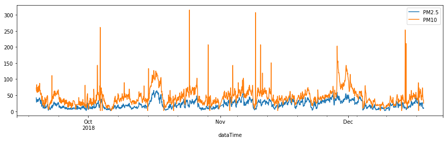
앞에서 계속 사용한 초미세먼지 데이터(PM2.5)에 미세먼지(PM10) 농도를 추가하여 Bivariate 시계열 예측을 수행해보도록 하겠습니다.
- 데이터 : 경남 창원시 의창구 원이대로 450(시설관리공단 실내수영장 앞)에서 측정된 초미세먼지(PM2.5)와 미세먼지(PM10)
- 기간 : 2018-9-18 19:00 ~ 2018-12-18 17:00 (3개월, 1시간 단위)
statsmodel의 VAR 모듈을 이용해 multivariate time sereis 모델링을 수행할 수 있습니다. VAR 모듈의 select_order 함수는 AIC, BIC, HQIC와 같은 지표를 기준으로 가장 최적의 order를 결정할수 있도록 도와줍니다. 최대 order를 30으로 하고 최적 order를 탐색한 결과, 아래와 같이 AIC 기준으로는 9, BIC 기준으로 5가 결정된 것을 볼 수 있습니다.
df = df[['pm10Value', 'pm25Value']]
model = sm.tsa.VAR(df, freq='H')
result = model.select_order(30, trend='nc')
print(result)
## <statsmodels.tsa.vector_ar.var_model.LagOrderResults object. Selected orders are: AIC -> 9, BIC -> 5, FPE -> 9, HQIC -> 5>
BIC 기준으로 order 5를 선택하여 모델을 학습한 결과는 아래와 같습니다. 모델이 추정한 파라미터를 이용해 수식으로 적어보면 다음과 같습니다.
\[\begin{align} \begin{bmatrix} X_t \\ Y_t \end{bmatrix} = & \begin{bmatrix} 0.227950 & 1.021808 \\ 0.013951 & 0.856883 \end{bmatrix} + \begin{bmatrix} X_{t-1} \\ Y_{t-1} \end{bmatrix} + \\ & \begin{bmatrix} 0.175133 & -0.172207 \\ 0.005520 & 0.090531 \end{bmatrix} + \begin{bmatrix} X_{t-2} \\ Y_{t-2} \end{bmatrix} + \\ & \begin{bmatrix} 0.114712 &-0.170387 \\ -0.000139 & -0.031543 \end{bmatrix} + \begin{bmatrix} X_{t-3} \\ Y_{t-3} \end{bmatrix} + \\ & \begin{bmatrix} 0.07475107 & -0.01361328 \\ -0.00297173 & -0.0174331 \end{bmatrix} + \begin{bmatrix} X_{t-4} \\ Y_{t-4} \end{bmatrix} + \\ & \begin{bmatrix} 0.16981114 & -0.20771503 \\ 0.00960018 & 0.03822593 \end{bmatrix} + \begin{bmatrix} X_{t-5} \\ Y_{t-5} \end{bmatrix} + \begin{bmatrix} Z_t \\ W_t \end{bmatrix}\end{align}\]results = model.fit(4, trend='nc')
print(results.summary())
  Summary of Regression Results
==================================
Model:                         VAR
Method:                        OLS
Date:           Mon, 14, Jan, 2019
Time:                     16:47:40
--------------------------------------------------------------------
No. of Equations:         2.00000    BIC:                    8.37752
Nobs:                     2179.00    HQIC:                   8.35103
Log likelihood:          -15249.5    FPE:                    4170.38
AIC:                      8.33576    Det(Omega_mle):         4139.93
--------------------------------------------------------------------
Results for equation pm10Value
===============================================================================
                  coefficient       std. error           t-stat            prob
-------------------------------------------------------------------------------
L1.pm10Value         0.246944         0.022176           11.136           0.000
L1.pm25Value         0.996998         0.096106           10.374           0.000
L2.pm10Value         0.200154         0.022561            8.872           0.000
L2.pm25Value        -0.199703         0.124451           -1.605           0.109
L3.pm10Value         0.147570         0.022565            6.540           0.000
L3.pm25Value        -0.191717         0.124290           -1.543           0.123
L4.pm10Value         0.113603         0.022163            5.126           0.000
L4.pm25Value        -0.040803         0.096037           -0.425           0.671
===============================================================================

Results for equation pm25Value
===============================================================================
                  coefficient       std. error           t-stat            prob
-------------------------------------------------------------------------------
L1.pm10Value         0.015231         0.005147            2.959           0.003
L1.pm25Value         0.856493         0.022305           38.399           0.000
L2.pm10Value         0.007163         0.005236            1.368           0.171
L2.pm25Value         0.087437         0.028884            3.027           0.002
L3.pm10Value         0.001760         0.005237            0.336           0.737
L3.pm25Value        -0.028244         0.028846           -0.979           0.328
L4.pm10Value         0.000100         0.005144            0.019           0.984
L4.pm25Value         0.023794         0.022289            1.068           0.286
===============================================================================

Correlation matrix of residuals
            pm10Value  pm25Value
pm10Value     1.000000   0.273513
pm25Value     0.273513   1.000000
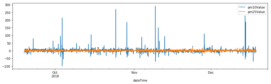
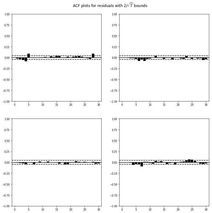
Univariate에서와 마찬가지로 모델의 적합성을 검증하기 위해 residual analysis를 수행합니다. residual plot과 residual acf 등을 그려 모델 적합성을 검증합니다. 두 시리즈의 residual acf가 거의 zero에 가가운 것을 볼 수가 있습니다.
results.resid.plot(figsize=(15,4))
plt.show()
results.plot_acorr(nlags=30, resid=True)
plt.show()
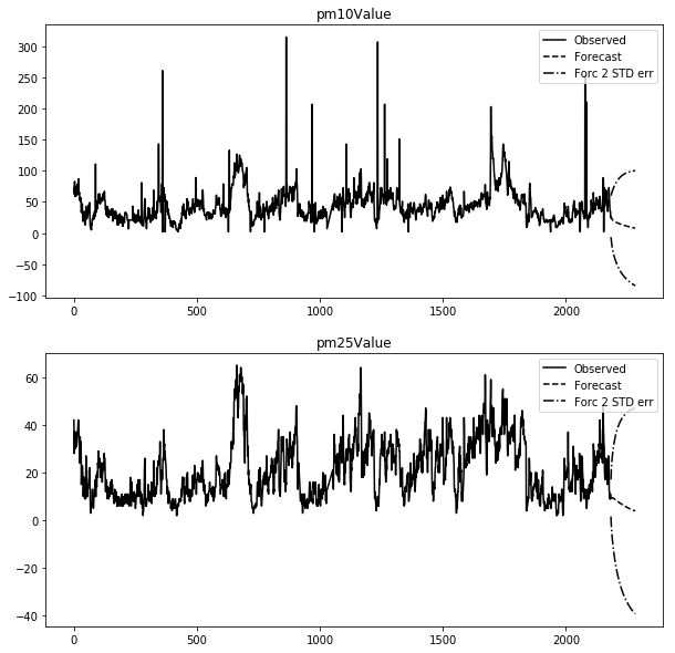
또한 plot_forecast 혹은 forecast 함수를 이용해 미래값을 예측할 수 있습니다.
results.plot_forecast(steps=100, alpha=0.05, plot_stderr=True)
plt.show()
Reference
[1] Introduction to Time Series and Forecasting, Peter J. Brockwell, Richard A. Davis,
Comments