
cs231n - 이해하기
cs231n
- http://cs231n.stanford.edu/
이 포스팅은 딥러닝에 대한 기본 지식을 상세히 전달하기보다는 간략한 핵심과 실제 모델 개발에 유용한 팁을 위주로 정리하였습니다.
activation functions
1) sigmoid
- saturated neurons kill the gradient
- sigmoid outputs are not zero-centered
2) tanh
- zero-cented but staturated neurons kill the gradient
3) relu
- doest not saturate
- computationally efficient
4) leaky relu
5) exponential Linear Units
Sigmoid outputs are not zero-centered. why is it problem?
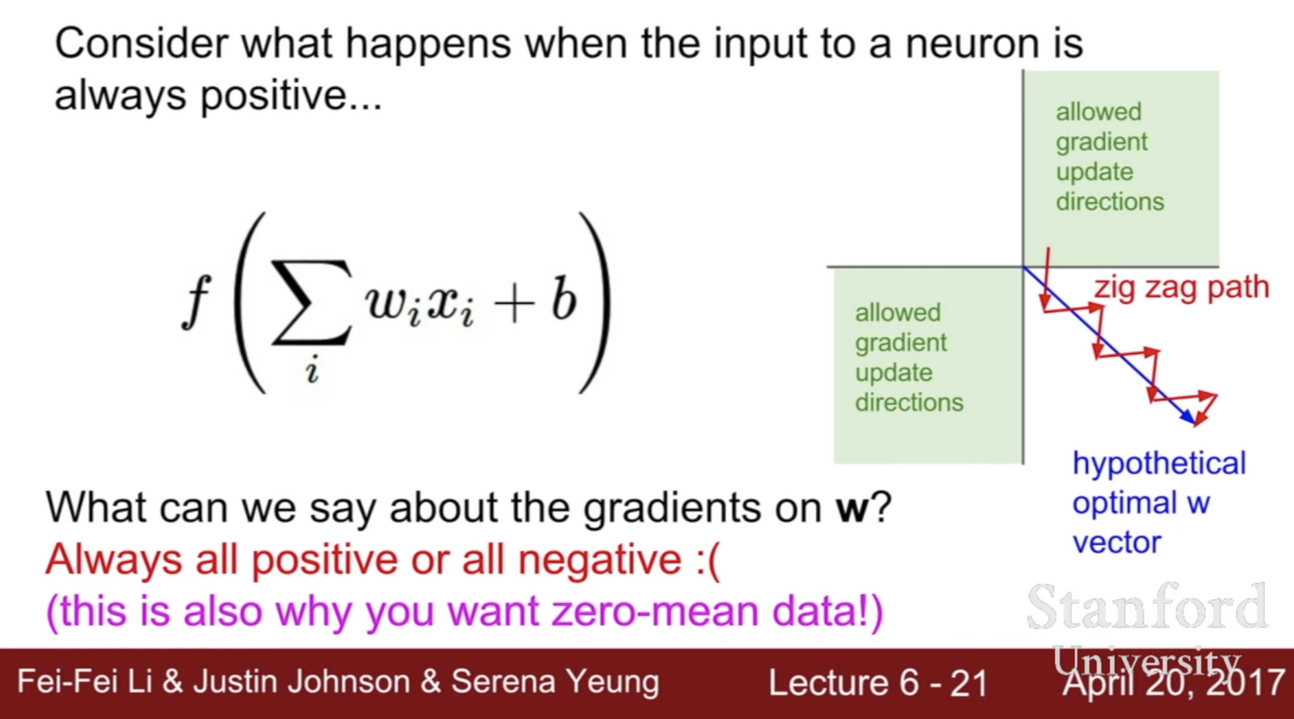
Sigmoid outputs are not zero-centered. This is undesirable since neurons in later layers of processing in a Neural Network (more on this soon) would be receiving data that is not zero-centered. This has implications on the dynamics during gradient descent, because if the data coming into a neuron is always positive (e.g. x>0 elementwise in f=wTx+b)), then the gradient on the weights w will during backpropagation become either all be positive, or all negative (depending on the gradient of the whole expression f). This could introduce undesirable zig-zagging dynamics in the gradient updates for the weights. However, notice that once these gradients are added up across a batch of data the final update for the weights can have variable signs, somewhat mitigating this issue. Therefore, this is an inconvenience but it has less severe consequences compared to the saturated activation problem above.
\[\frac{dL}{dw} = \frac{dL}{df}\frac{df}{dw}\\ \frac{df}{dw} = x \ and \ x \ are \ all \ positive,\\ the \ gradient \frac{dL}{dw} \ always \ has \ the \ same \ sign \ as \frac{dL}{df} \ (all \ positive \ or \ all \ negative )\]Nesterov Momentum
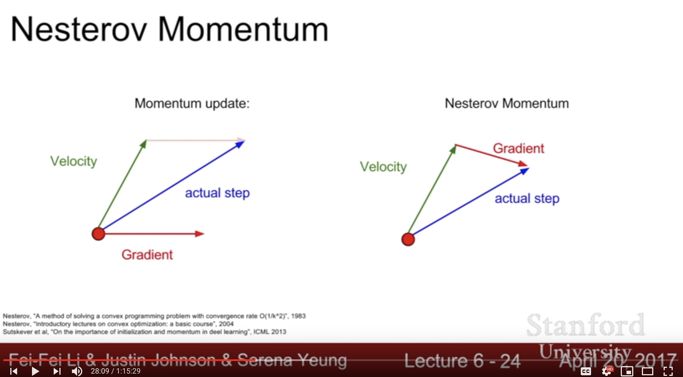
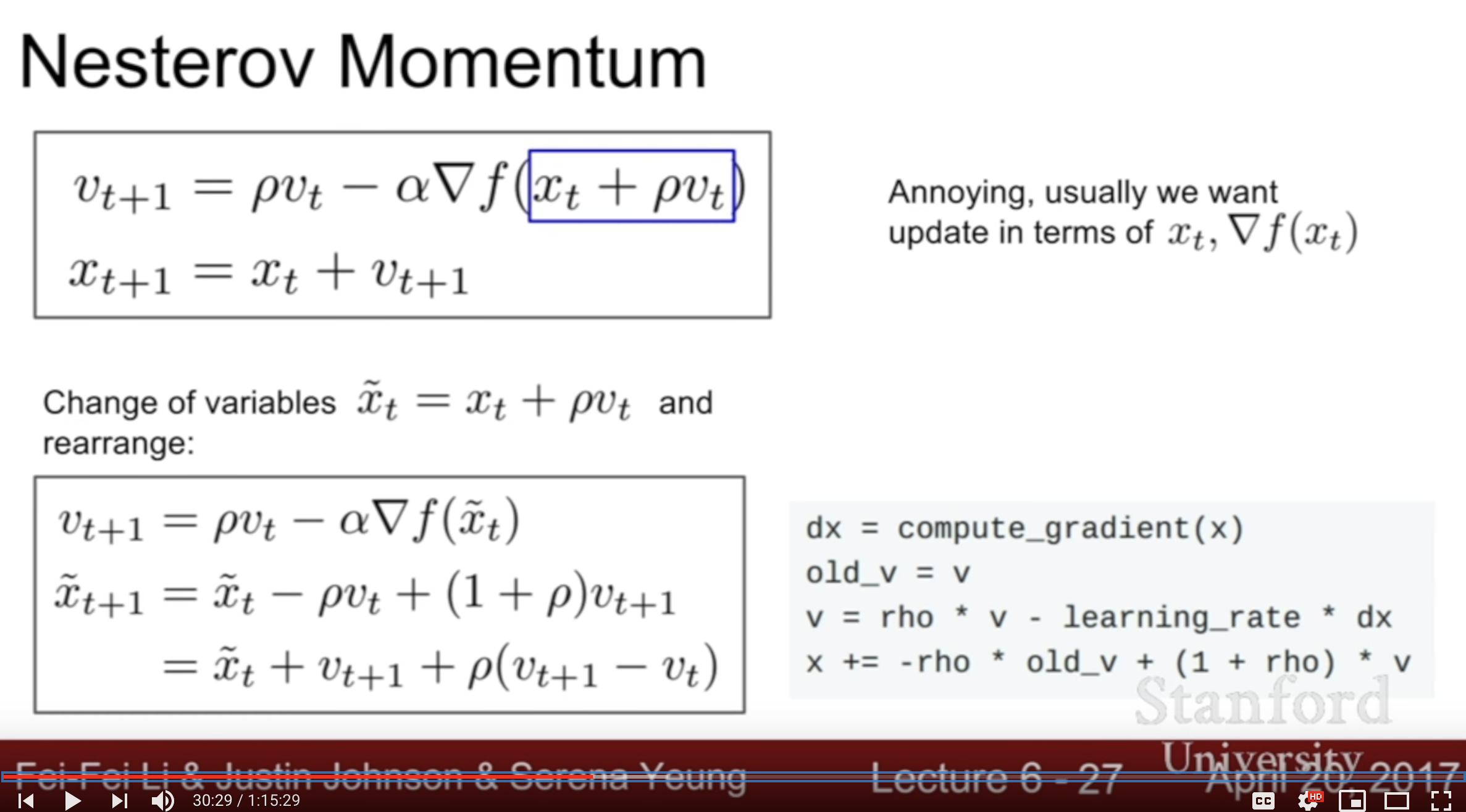

현재 위치의 그래디언트 g(\(\theta_t\)) 를 이용하는 것이 아니고 현재 위치에서 속도 \(\mu v_t\)만큼 전진한 후의 그래디언트 g(\(\theta_t + \mu v_t\)) 를 이용합니다. 사람들은 이를 가리켜 선험적으로 혹은 모험적으로 먼저 진행한 후 에러를 교정한다라고 표현합니다. (ref : https://tensorflow.blog/2017/03/22/momentum-nesterov-momentum/)
optimizer
1) SGD
while True :
  dx = compute_gradient(x)
  x += -learning_rate * dx
2) SGD + Momentum
vx = 0
while True :
  dx = compute_gradient(x)
  vx = rho * vx + dx
  x += -learning_rate * vx
3) Nesterov Accelerated Gradient(NAG)
vx = 0
while True :
  dx = compute_gradient(x)
  old_vx = vx
  vx = rho * vx - learning_rate * dx
  x += -rho * old_vx + (1 + rho) * vx
4) AdaGrad
grad_squared = 0
while True :
  dx = compute_gradient(x)
  grad_squared += dx * dx
  x += -learning_rate * dx / (np.sqrt(grad_squared) + 1e-7)
5) RMSProp
grad_squared = 0
while True :
  dx = compute_gradient(x)
  grad_squared += decay_rate * grad_squared + (1-dacay_rate) * dx * dx
  x += -learning_rate * dx / (np.sqrt(grad_squared) + 1e-7)
6) Adam
first_moment = 0
second_moment = 0
for t in range(num_iterations):
  dx = compute_gradient(x)
  first_moment = beta1 * first_moment + (1-beta1) * dx
  second_moment = beta2 * second_moment + (1-beta2) * dx * dx
  ## bias correction for the fact that first and second momentum estimates start at zero
  first_unbias = first_moment / (1-beta1 ** t)
  second_unbias = second_moment / (1-beta2 ** t)
  x -= learning_rate * first_moment / (np.sqrt(second_moment) + 1e-7)
#### Tips!!
## Adam with bete1 = 0.9 and beta2 = 0.999 and
## learning_rate = 1e-3 or 5e-4 is a great starting point
## for many models!
옵티마이저에 상관없이 모두 learning rate 하이퍼파라미터가 필요함. 어떻게 조절하지? decay over time!
- SGD with Momentum에서는 흔히 사용. 하지만 Adam에서는 잘 사용안함.
- second order hyperprameter임. First, try no decay and see what happen.
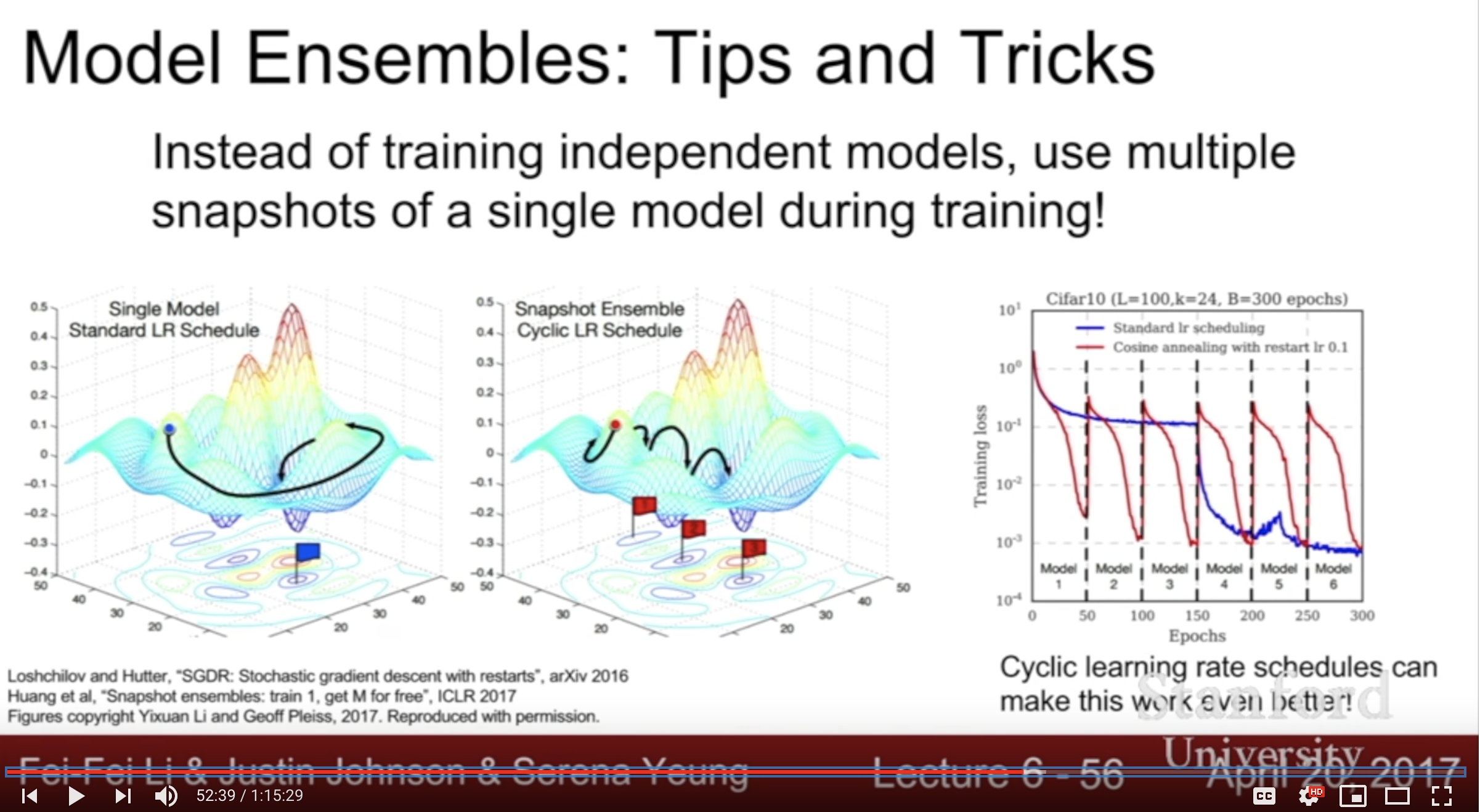
Model ensembel trick
- Enjoy 2% extra performance
- 독립적인 모델을 여러개 만드는 것보다 한가지 모델의 여러 스냅샷을 앙상블하는게 효과적.
regularization
common pattern : add random noise in train, marginalize over the noise in test
1) Dropout 2) Batch Normalization 3) Data Augmentation – below is not common in practice, but cool ideas 4) DropConnect - 랜덤하게 activation값을 제로로 만드는 dropout과 비슷. 하지만 activation이 아니라 weight를 제로로 만드는 것 5) Fractional max pooling - 풀링레이어에서 풀링 영역을 랜덤하게 선택 6) stochastic depth - 전체 레이어 중 랜덤하게 선택한 레이어만 학습. 테스트할때는 averaging하여 전체를 사용
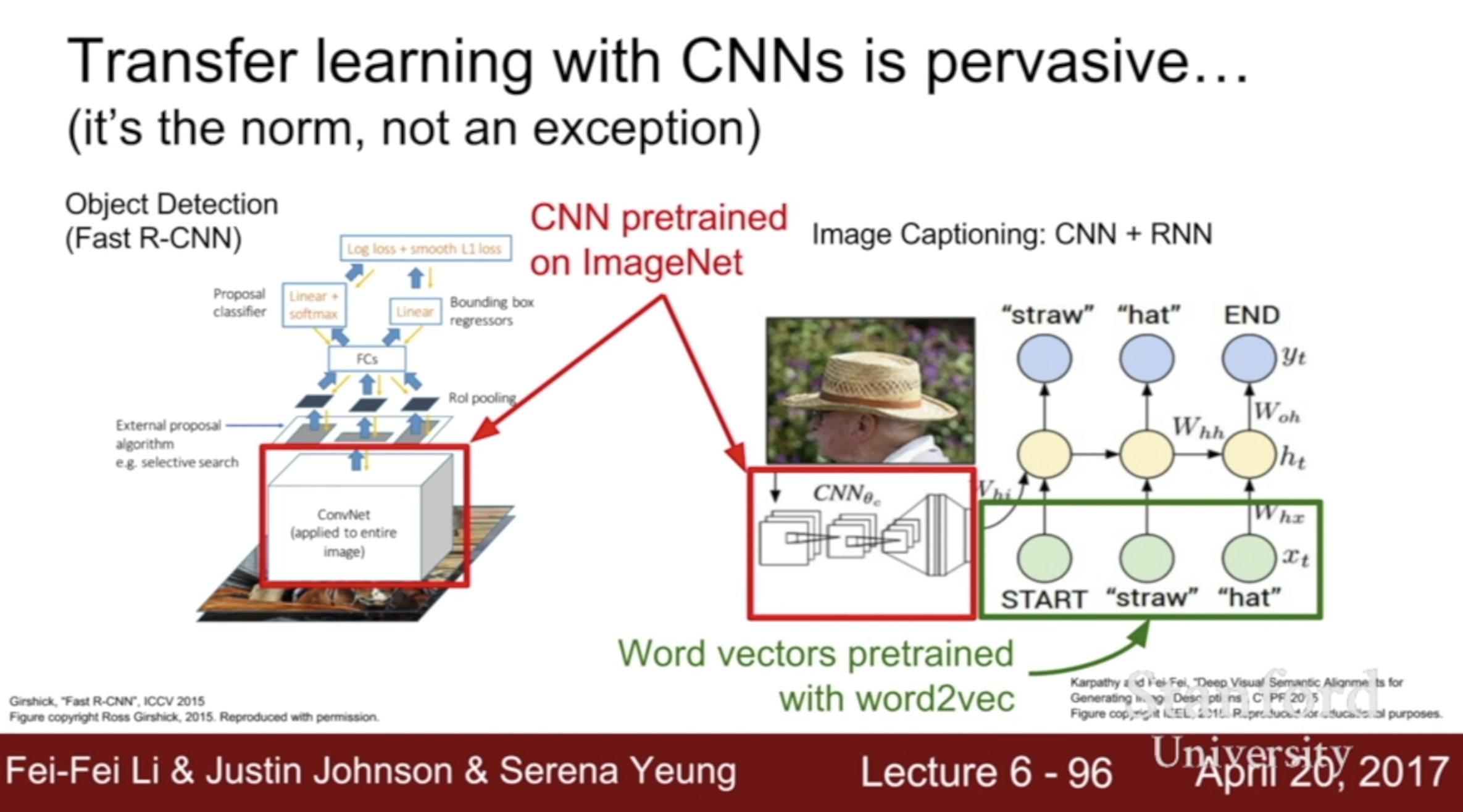
transfer learning
- It’s the norm, not the exception
| very similar dataset | very different dataset | |
|---|---|---|
| very little data | Use Linear Classifier on top layer | you’re in trouble.. Try linear classifier from different stages |
| quite a lot of data | Finetune a few layers | Finetune a larger number of layers |
CNN architectures
1) Lenet-5
2) AlexNet - 7x7 filter size
3) VGG - 3x3 filter size
- why use smaller filters? (3x3 conv)
- stack of three 3x3 conv (stride 1) layer has same effective receptive field as one 7x7 layer
- But deeper, more non-linearities
- And fewer parameters: 3 * (32C2) vs. 72C2 for C channels per layer
4) GoogLeNet
- Inception module : 1x1 conv, 3x3 conv, 5x5 conv and 3x3 pooling in parallel –> concatenate outputs
- computational expensive
- adding 1x1 conv(64 filter) as bottlenecks
- auxiliary classification outputs to inject additional gradient at lower layers
5) ResNet
– below others to know
6) Network in Network (NiN)
- philosophical inspiration for googLeNet
7) Wide Residul Networks
- residuals are the important factor, not depth
- Use wider residual blocks (F x k filters instead of F filters in each layer)
- 50-layer wide resnet outperforms 152-layers original resnet
8) deep networks with stochastic depth
- randomly drop a subset of layers during each training pass
9) FractalNet
10) Densely connected conv net
- each layer is connected to every other layer in feedforward fashion
RNN
- one to one - vanilla NN
- one to many - image captioning
- many to one - sentiment classification
- many to many - machine translation
- many to many - video classfiction on frame level
backpropagation through time is super slow!
Truncated Backpropagation through time
minibatch별로 나눠서 그래디언트 업데이트
1) Image captioning
- input : image -> ConvNet -> FC 4096
- take FC 4096 as first hidden state vector
2) Image captioning with Attention
- 이미지의 location 정보를 이용하도록 함
3) Visual Question Answering : RNN with Attention
vanilla RNN gradient flow
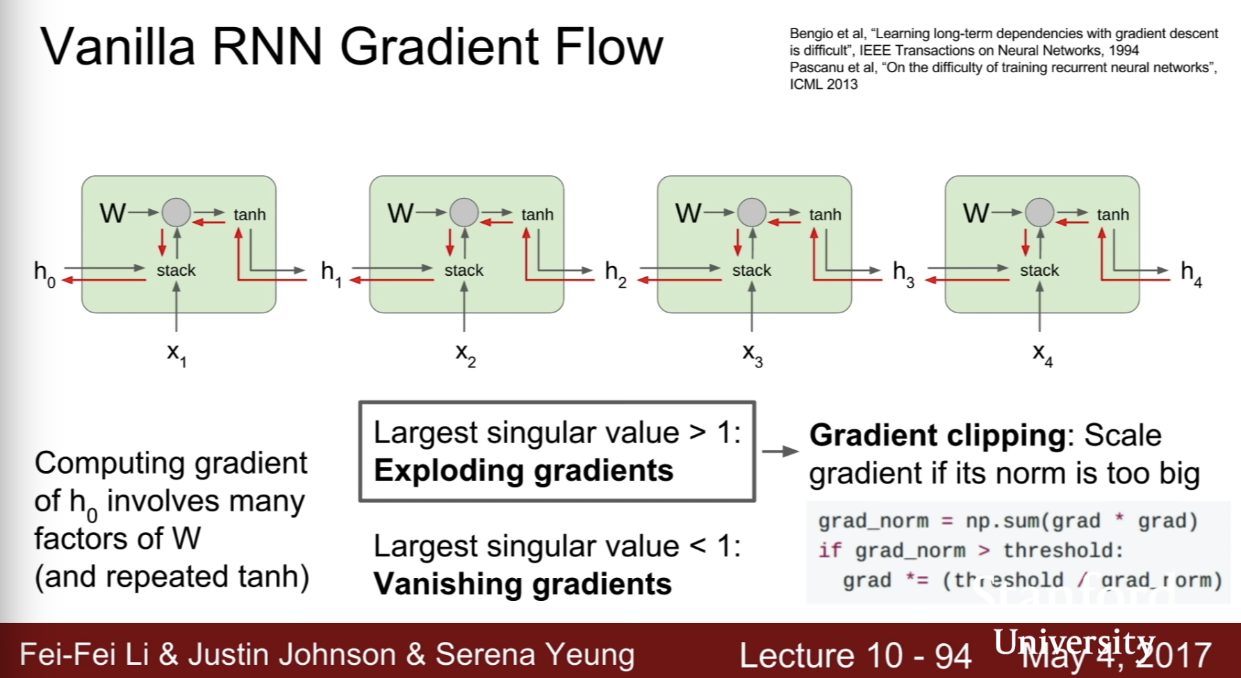
computing gradient of h0 involves many factors of W
- exploding gradients -> gradient clipping
- vanishing gradients -> change RNN architecture (LSTM)
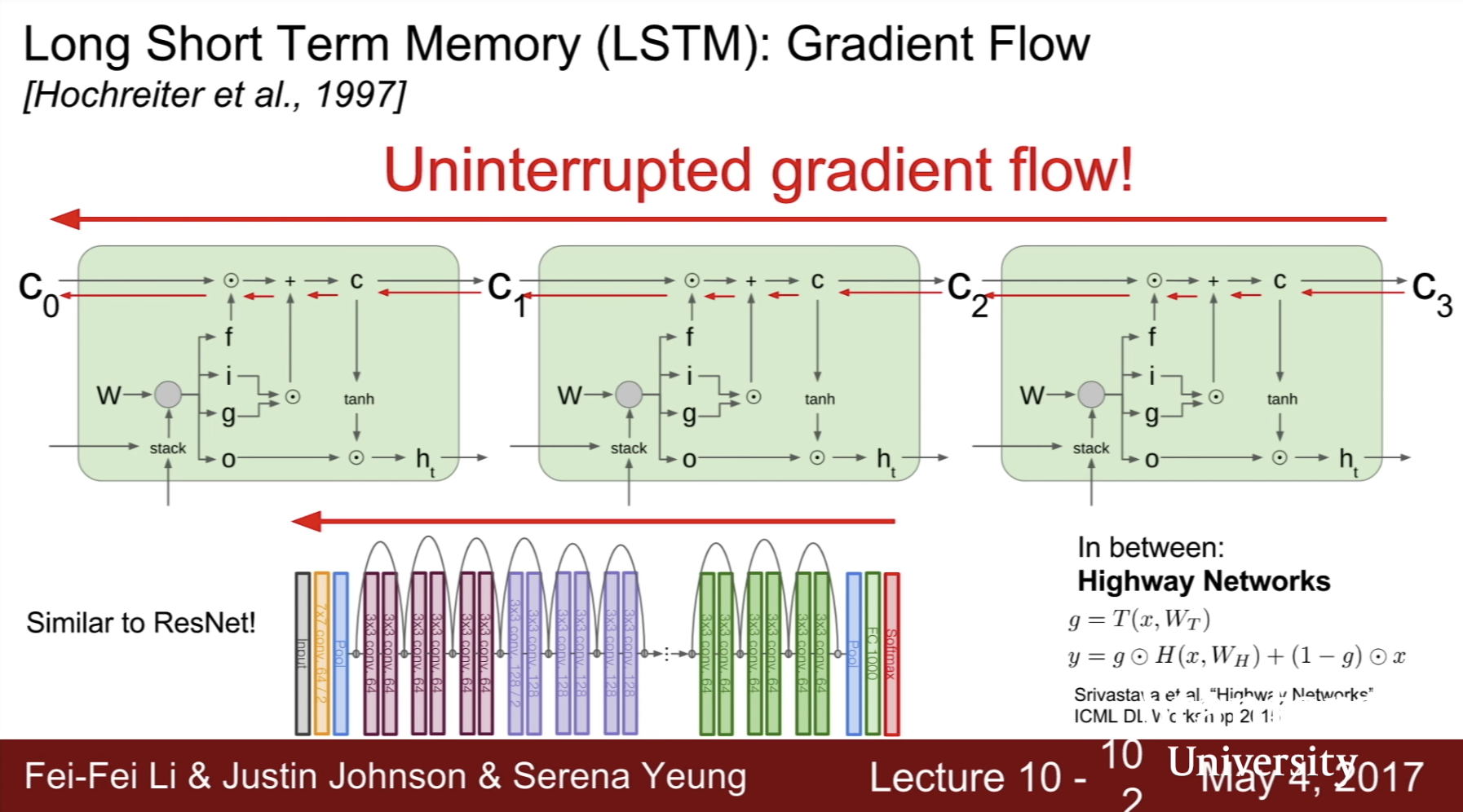
LSTM
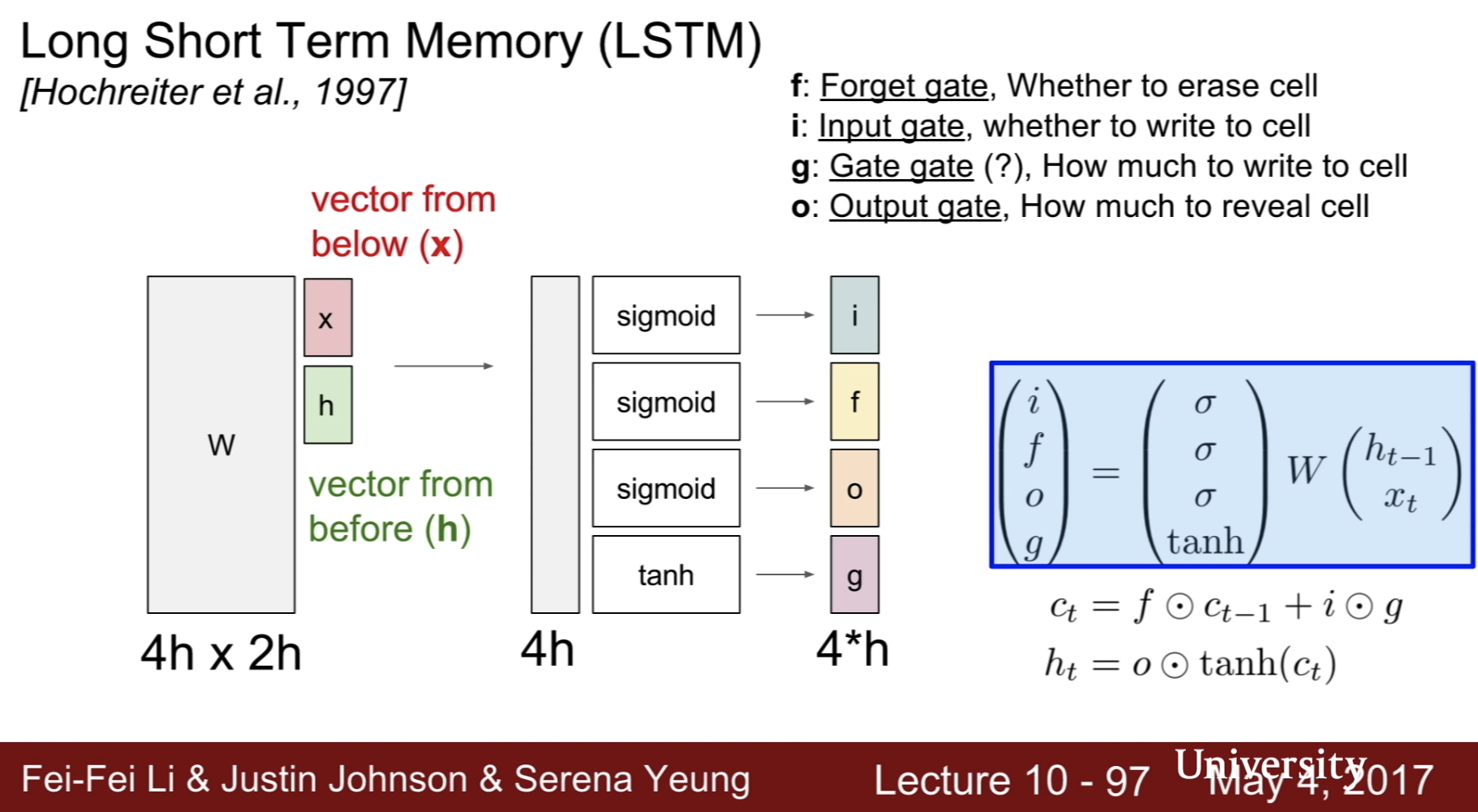
- i, f, o, g gate
- forget gate : whether to erase cell
- input gate : whether to wirte to cell
- gate gate : how much to wirte to cell
- output gate : how much to reveal cell
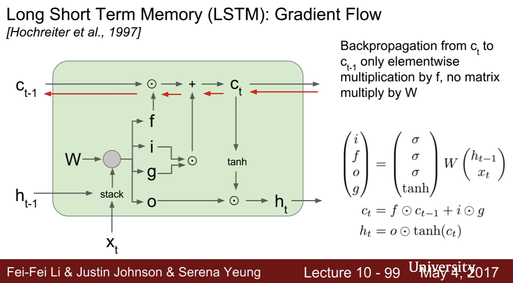
backpropagation from ct to ct-1 only elementwise multiplication by f, no matrix multiply by W
Comments