cs231n - 이해하기 2
cs231n
- http://cs231n.stanford.edu/
이 포스팅은 딥러닝에 대한 기본 지식을 상세히 전달하기보다는 간략한 핵심과 실제 모델 개발에 유용한 팁을 위주로 정리하였습니다.
Detection and Segmentation
1) semantic segmentation :
- sliding window
- Fully convolutional : labeling class per every pixel
- downsampling and upsampling : how to upsampling(unpooling)
- nearest neighbor
- bed of nails
- max unpooling(remember which element was max)
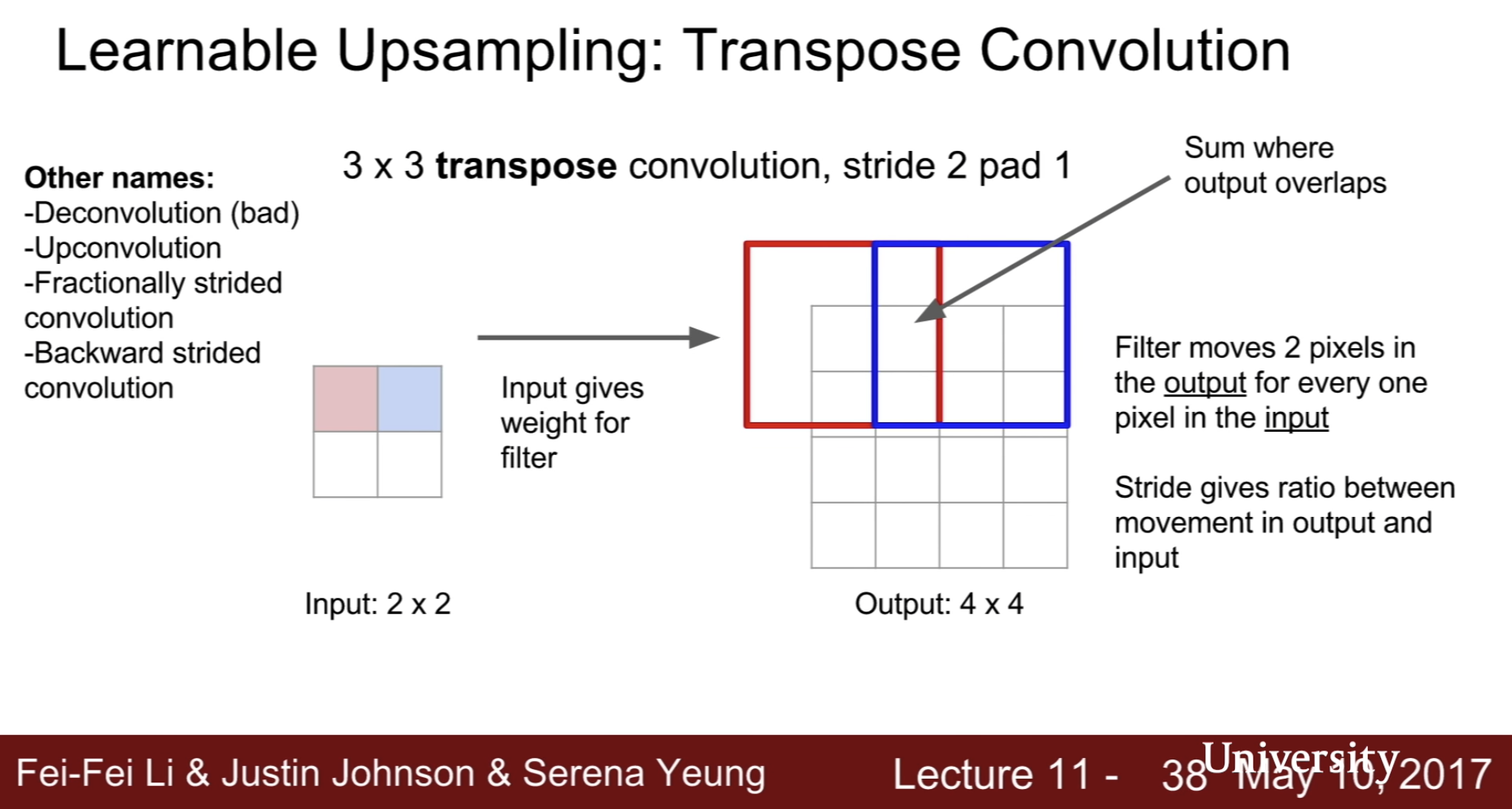
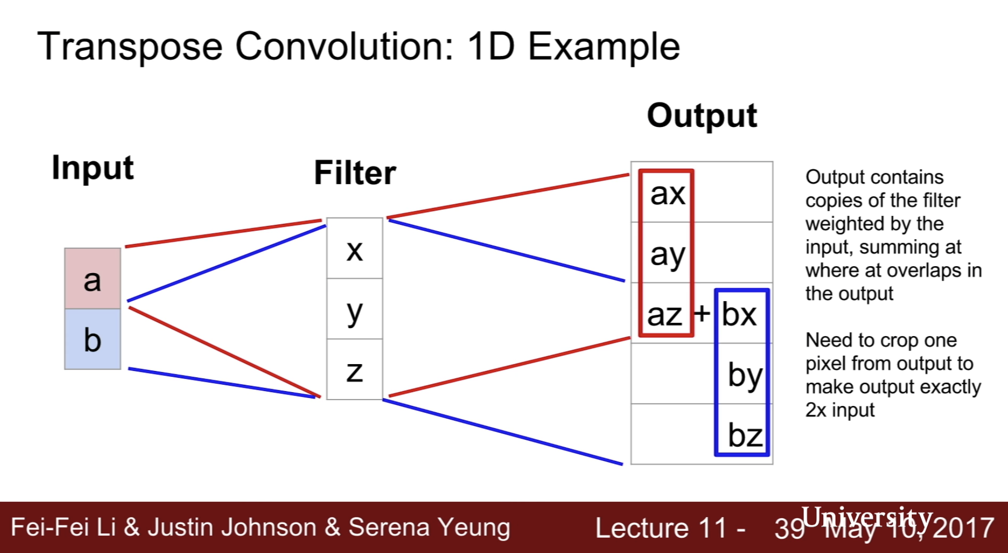
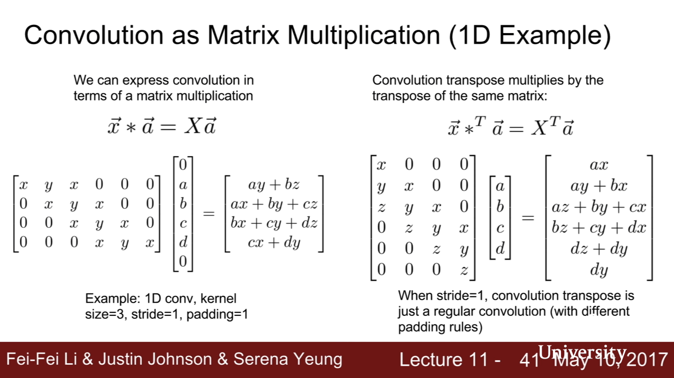
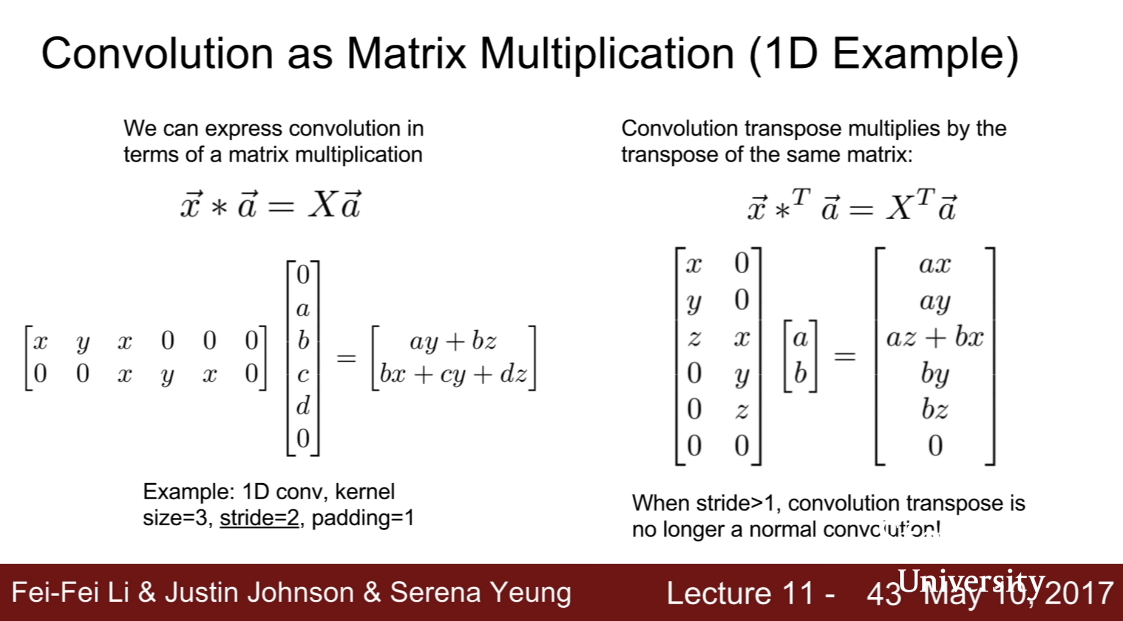
- Transpose Convolution
- downsampling and upsampling : how to upsampling(unpooling)
2) classification + localization :
- class score : softmax loss
- box coordiantes(x, y, w, h) : L2 loss
- treat localization as a regression problem
multimodal - how to determine weight of two different loss function? loss값 외에 다른 지표를 참고
- aside : Human pose estimation
3) Object Detection
- fixed set of categories and draw box location
- benchmark dataset : PASCAL VOC
- each image needs a different number of outputs - not easy to solve with regression
- sliding window : crops of the image, CNN classifies each crop as object or background
- how to choose crop? need to apply CNN to huge number of locations and scales very expensive
- region proposals : selective search gives 1000 region proposal -> brute force but high recall
- R-CNN
- region of interest(RoI) from a proposal method (~2k)
- Warped image regions
- forward each region through convNet
- classify regions with SVMs
- Box regression
slow train and inference
- fast R-CNN
- Forward whole image through ConvNet
- RoIs from proposal method on convnet feature map of image
- RoI pooling layer
- fully connected
- classification and regression
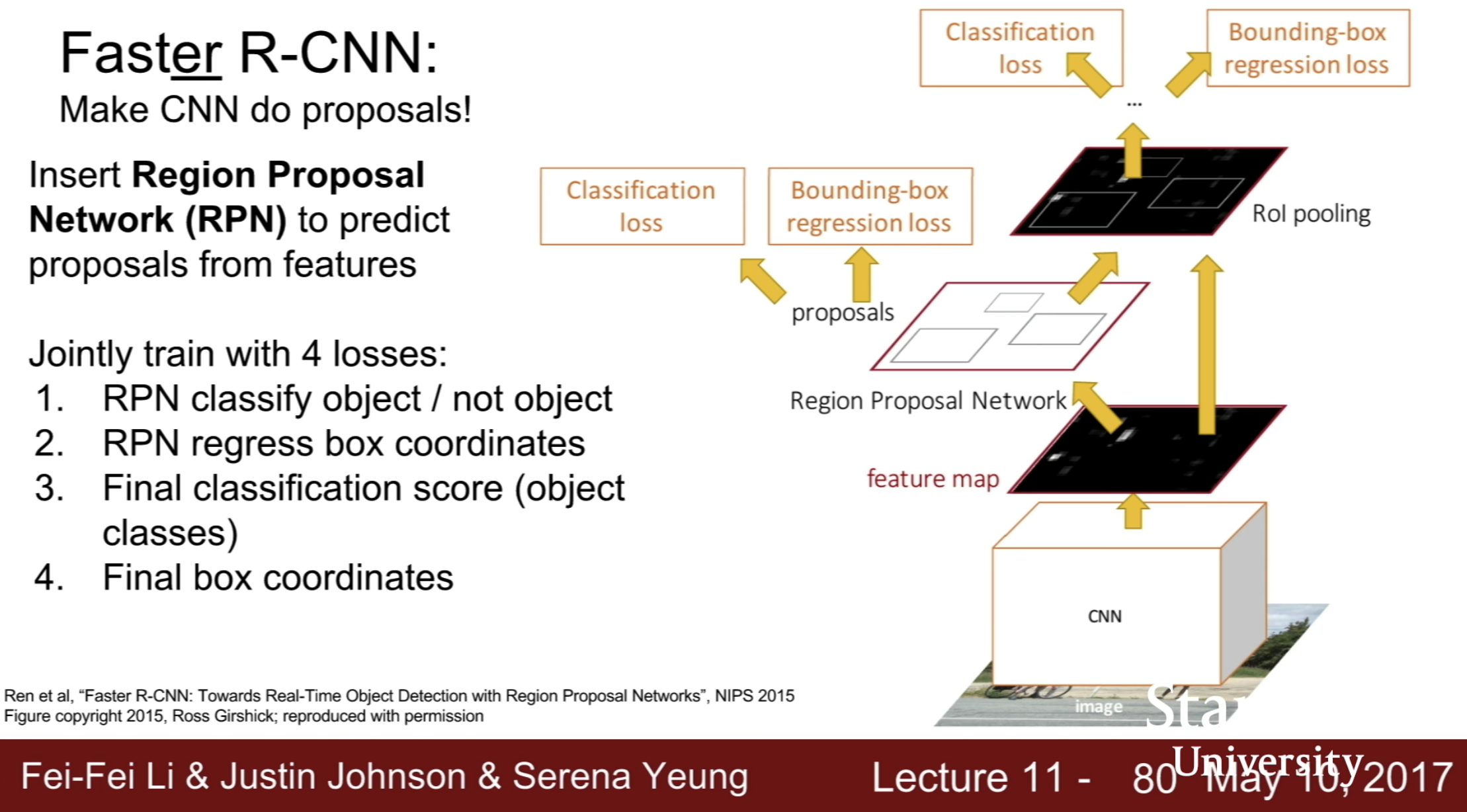
- faster R-CNN
- make CNN do proposals
- insert region proposal network(RPN) to predict proposals from features
- jointly train with 4 lossess
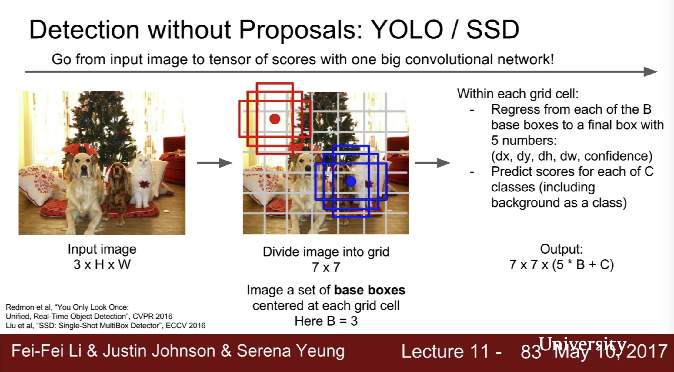
- detection without proposals : YOLO / SSD
4) Instance Segmentation
- Mask R-CNN - similar to faster R-CNN
- can also does pose : add joint coordinates
- bechmark data : microsoft coco data
Visualizing and Understanding
what’s going on inside ConvNets? What are the intermediate features looking for?
- visualize the filters : raw weights
- not that interesting
- Last Layer :
- check Nearest Neighbors in faeture space(last fc layer)
- dimensionality reduction : PCA, t-SNE
- Occlusion Experiments : 부분적으로 마스크함
- mask한 영역으로 인해 확률이 극격히 변화면 해당 영역은 크리티컬하다고 가정
- saliency maps : 이미지의 각 픽셀들에 대해서 클래스 스코어의 그래디언트를 구함. compute gradient of class score with respect to image pixels
- intermediate feature via guided backprop : which part of image impact to intermediate activation value
- relu : positive gradient만 이용하면 더 나이스 이미지를 얻을수 있다
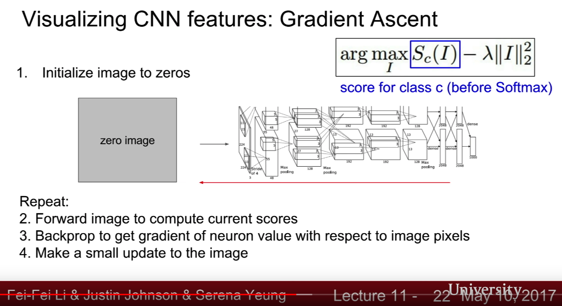
- gradient ascent : 지금까지는 보통의 백프로파게이션을 통해 이미지의 어떤 부분이 뉴련에 영향을 주는지 알아봤다면(고정된 입력 이미지 값), 그래디언트 어센트는 뉴런의 액티베이션을 최대화하는 방향으로 이미지를 만들어내는 것임(입력 이미지 값을 생성하는 것)
- generate a synthetic image that maximally activates a neuron
- better regrularizer (image prior regualarization)
- optimize in FC6 latent space instead of pixel space
- Fooling Image
- 엘리퍼튼 이미지를 고르고
- 코알라 클래스 스코어를 골라
- 코알라 클래스 스코어를 최대화하도록 이미지를 모디파이
- 네트워크가 코알라로 분류할때까지 반복
- DeepDream
- choose an image and a layer in a CNN : repeat:
- Forward : compute activations at chosen layer
- set gradient of chosen layer equal to its activation
- backward : compute gradient on image
- update image
- choose an image and a layer in a CNN : repeat:
- Feature Inversion : 피쳐벡터를 뽑고, 그 피쳐벡터에 매칭되는 다른 입풋 이미지를 만들어냄

- Texture sythesis : given a sample patch of some texture, can we genrate a bigger image of the same texture?
- classical approch : nearest
- neural texture synthesis : gram matrix
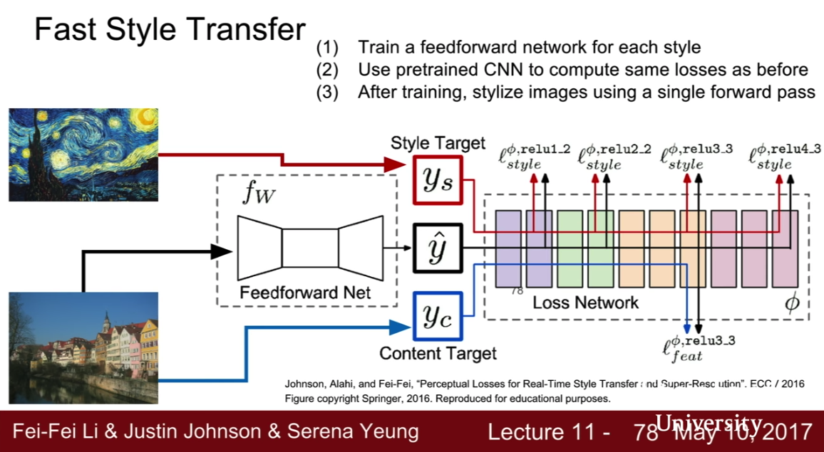
- Style Transfer
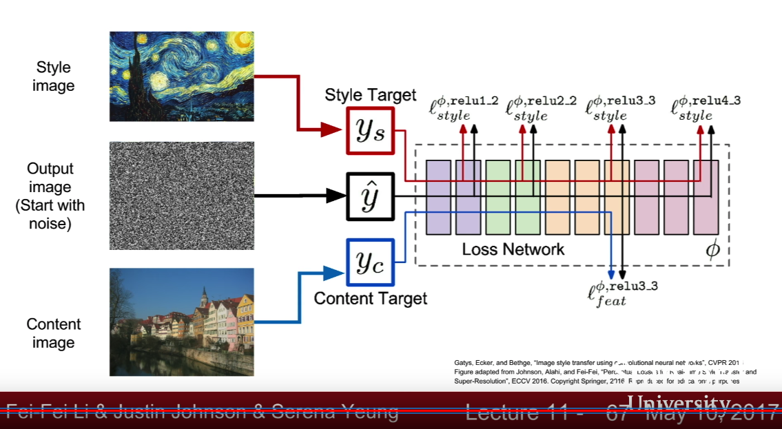
- slow : train another model to transfer style
- fast style transfer
Generative Models
- addresses density estimation
-
generative models of time-series data can be used for simulation and planning
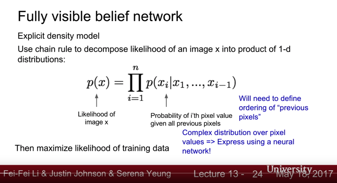
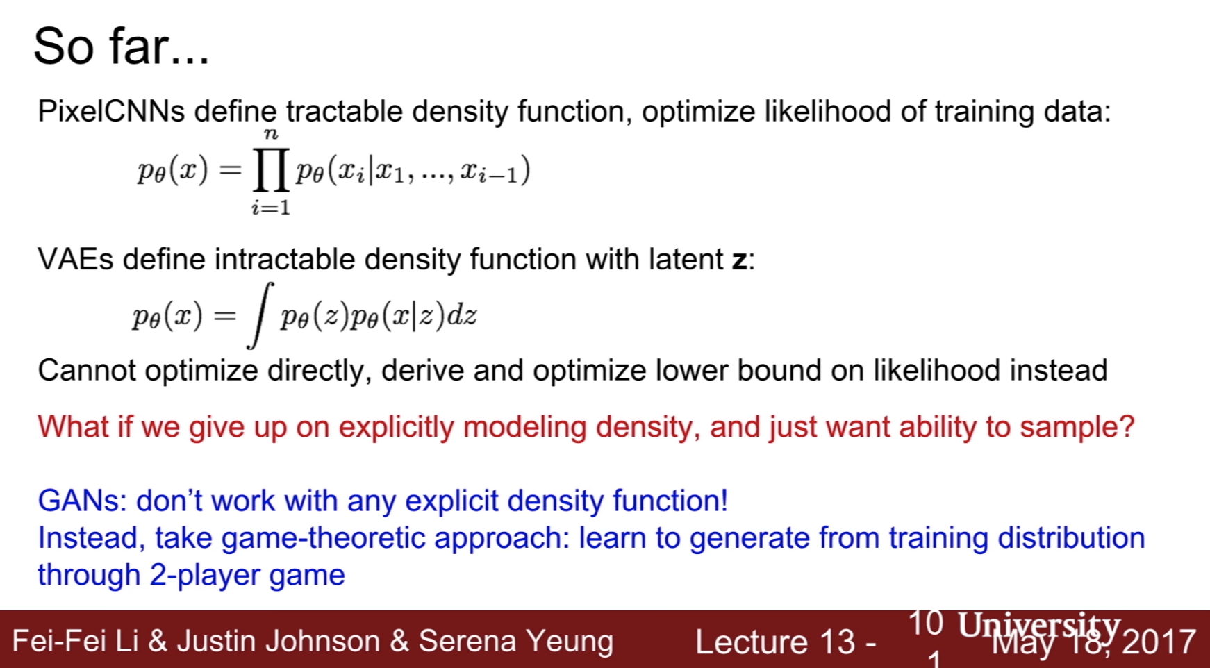
- Fully visible belief network
-
픽셀의 오더를 어떻게 결정하지? –> pixelRNN
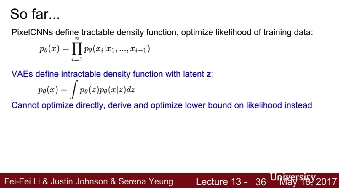
- pixelRNN
- 코너에 있는 픽셀부터 다이어고날 방향으로 시퀄셜로 학습 using RNN (LSTM)
- sequtional is slow
- pixelCNN
- 코너에 있는 픽샐부터 시작하는 것은 같으나
- context region(previous pixels)으로부터 모델링되는 것
- training is faster but generation must still process sequentially
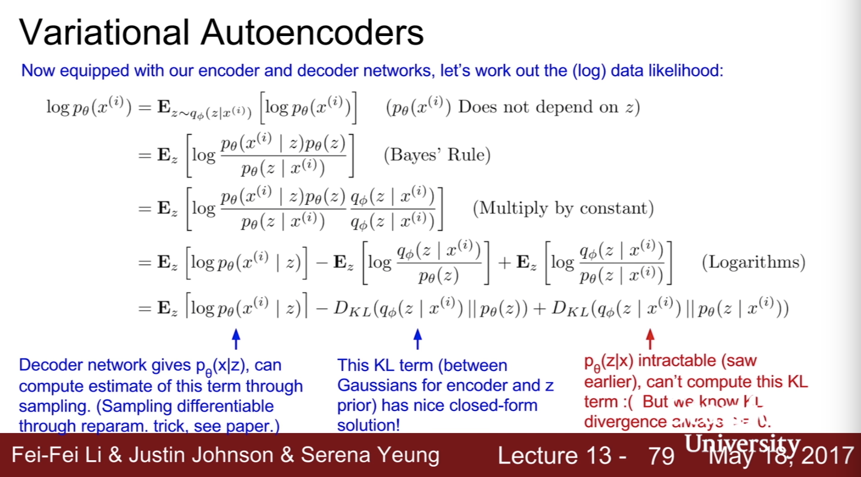
- Variational auto-encoder
- intractible to compute p(x|z) for every z
- in addition to decoder pθ(x|z), define additional encoder qφ(z|x) that approximates pθ(z|x)
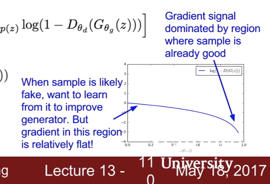
- GAN


Comments